Improved Distributed Estimation Method for Environmental
time-variant Physical variables in Static Sensor Networks
Magdi S. Mahmoud, Haris M. Khalid and Muhammad Sabih∗†
March 15, 2013
Abstract
In this paper, an improved distributed estimation scheme for static sensor networks is developed. The scheme is developed for environmental time-variant physical variables. The main contribution of this work is that the algorithm in [1]-[3] has been extended, and a filter has been designed with weights, such that the variance of the estimation errors is minimized, thereby improving the filter design consid-erably and characterizing the performance limit of the filter, and thereby tracking a time-varying signal. Moreover, certain parameter optimization is alleviated with the application of a particular finite impulse response (FIR) filter. Simulation results are showing the effectiveness of the developed estimation algo-rithm.
Keywords:Distributed estimation, static sensor networks, minimum variance, performance limit,
param-eter optimization, estimation algorithm, time-variant.
1
Introduction
A sensor network (SN) is a network of autonomous devices that can sense their environment, make computa-tions and communicate with neighboring devices. SNs and in particular wireless sensor networks (WSNs), have a growing domain of application in areas such as environmental monitoring, industrial automation, intelligent buildings, search and surveillance, and automotive applications [4]-[11]. The characteristics of SNs motivate the development of new classes of distributed estimation and control algorithms which explore these systems limited power, computing and communication capabilities. It is important that the algorithms have tuning parameters that can be adjusted according to the demands set by the applications. In this paper, we investigate a distributed estimation algorithm for tracking an unknown time-varying physical variable.
Today, an increasing number of applications demands remote control of plants over unreliable networks. In these systems issues of communication delay, data loss and time–synchronization play critical roles. It is noted in [12] that several approaches have focused on diffusion mechanisms to have each node of the network obtain the average of the initial samples of the network nodes. Major progress has been made in understanding the convergence behavior of these consensus or state-agreement approaches. In [1], a scheme
∗ManuscriptMsM-KFUPM-HK-MS[R-III].tex
†Systems Engineering Department, King Fahd University of Petroleum and Minerals, P. O. Box 5067, Dhahran 31261,Saudi
for sensor fusion based on a consensus filter is proposed. Here, each node computes a local weighted least squares estimate that is shown to converge to the maximum likelihood solution for the overall network.
This paper is organized as follows. Section 2 presents the related works. Section 3 presents the distributed estimation problem formulation considered throughout the paper. The distributed estimator design is dis-cussed in Section 4. A distributed minimum variance optimization problem is posed and by restricting the set of admissible filter weights, it is possible to obtain a solution where the error convergence is guaranteed. A bound on the estimation error variance is also computed. The latter part of Section 4 discusses estimation of the error covariance. Section 5 presents the detail of the implementation of the estimation algorithm. Numerical results and implementation structure illustrating the performance of the proposed estimator and comparing it to some related proposals are also given. Finally, Section 6 concludes the paper.
2
Related Works
An extension of the approach for development of consensus filter based on sensor fusion is presented in [13], where the authors study a distributed average computation of a time-varying signal, when the signal is affected by a zero-mean noise. A convex optimization problem is posed to compute the edge weights, which each node uses to minimize the least mean square deviation of the estimates. The same linear fil-ter is also considered in [14], where the weights are computed off-line to speed up the computation of the averages. Another approach towards estimation is using H∞ estimation with the case of limited commu-nication capacity [15] and asynchronous filtering in [16]. Further characterization of consensus filters for distributed sensor fusion is given in [3]. Another approach to distributed estimation is based on nonlinear filters using self-synchronization and coupling functions, see [17]-[20]. In this case, the estimate of each node is provided by the state of a nonlinear dynamical system. This system is coupled to some of the other nodes by a static coupling function. Some conditions on the coupling function that lead to asymptotic state synchronization are investigated in [20]. Distributed filtering using model-based approaches is studied in various wireless network contexts, see for example [21]-[25]. Distributed Kalman filters and more recently a combination of the diffusion mechanism, discussed previously, with distributed Kalman filtering, see [2] and [26] have been proposed. A plausible approach is to communicate the estimates of the local Kalman filters, and then average these values using a diffusion strategy.
Distributed signal processing is a very active research area due to the recent developments in networking, computer and sensor technologies. In-network computing thus differs from the traditional architecture where sensors simply provide raw data to a fusion center. By letting the network do the computations, it is possible to reach a scalable, fault tolerant and flexible design. The drawback is that such a system is more difficult to analyze, as it is an asynchronous distributed computing system [27] with inputs and dynamics coupled to a physical environment. Despite current research activity and major progress, the theoretical understanding is far from satisfactory of these systems, exposed to link and node failures, packet drops, restricted power consumption, to name a few.
sufficient statistics over the entire network through communication with neighbor nodes is shown in [34]. Ignoring this, time delay is an obvious violation of the physics behind the propagation of signal, being envisioned to be best estimated from measurements of distantly placed sensor nodes. Some recent results on various topics of distributed estimation have been reported in [35]-[41]. If we consider results on time-vary-ing state delay on network systems, an approach can be seen in [42]. Also, a robustH∞estimation with signal transmission delay and data packet dropouts can be seen in [43]. Moreover, considering the work on time-delay a new delay system on networked system is proposed in [44], a robust stability for uncertain delay in [45], a stabilization approach with delay in [46] and [47], a filtering technique for mixed random delays is shown in [48], a feedback control approach with mixed delays is working in [49] and a disturbance rejection technique for discrete-time delay systems is shown in [50].
The problem statement for estimation physical variables in SNs can be stated as follows. Consider the estimation of an available SN is to be based on the available sensor measurements. In sensor networks, due to the constraints on communication and computation, we cannot broadcast all the sensor measurements to implement the real-time estimation of the field at the locations of interest. Rather, we have to determine the relevant sensors and use their particular measurements only in the field estimation at a particular location of interest.
The new proposed estimator for SNs presented in this paper belongs to a class of recently developed filtering algorithms that exploit in-network computing [12]. The scalability of these algorithms is based on that node operates using only local information. Suitable cooperation between neighboring nodes improves the estimation quality considerably. Using sensor readings from more than one sensor, for example, can overcome intrinsic performance limitations due to uncertainty and noise present in individual devices.
In this paper, we adopt the concept of minimum variance to develop an improved distributed estimation algorithm by considering the propagation delay of the physical quantity to be measured. This estimation algorithm has the following features:
• With a consideration of time-delay appearing in the measurements of different sensor nodes, it is assumed that the source of data is located at a known position.
• It incorporates an FIR filter aims at simplifying the signal estimation and alleviating the parameter optimization.
• It tracks a time-varying signal, while the estimators of [51] and [1] are limited to averaging initial samples.
• Our approach does not require a model of the system that generates the signal to track, in contrast to model-based approaches [2] and [25].
• There is no pre-assigned coupling law imposed among the nodes as in [20].
• Compared to the methods of [1]–[3], our approach does not rely on the Laplacian matrix associated with the communication graph. Rather, it considers a more general model of the filter structure. • Our filter parameters are computed through distributed algorithms, whereas, for example, the
estima-tors of [13] and [14] rely on centralized algorithms for designing the filters.
Remark 2.1 In this paper an improved distributed estimation method will be developed based on the con-cept of minimum variance with a consideration of time delay appearing in the measurements of different sensor nodes. The scheme is developed on a static SN. This is attributed to the time taken by physical quan-tity to be measured (for example, temperature, acoustic waves, to name few) to propagate from one point in the space to another one. In this regard, it is assumed that source of the data is located at a known position and the spatial ordinates of the sensor nodes are known. This knowledge is applied to calculate the time delay between the source of the data and any node in the network. The spectrum of the signal of interest is assumed to be known a–priori. Based on this knowledge the data is first passed through a low pass FIR filter. The signal is then jointly tracked by a SN, in which each node computes an estimate as a delay adjusted weighted sum of its own and its neighbors measurements and estimates. The filter weights are time varying and updated locally and it has a cascade structure comprised of two loops: an inner loop producing the state estimate and an outer loop producing an estimate of the error covariance. The state estimate is thus obtained as the solution of an optimization problem with quadratic cost function and quadratic constraints. As will be shown in later section, incorporation of FIR filter helps to alleviate the optimal estimation of a parameter, at a cost of acceptable deviation from the otherwise regular estimate. We show that the problem has a distributed implementation with conditions that can be locally checked. It is argued that the estimator is practically stable if the signal to track is slowly varying, so the estimate of each node converges to a neigh-borhood of the signal to track. The estimate in each node has consequently a small variance and a small bias. A bound on the estimation error variance, which is linear in the measurement noise variance and de-cays with the number of neighboring nodes, is presented. The algorithm is thus characterized by a trade-off between the amount of communication and the resulting estimation quality. Compared to similar distributed algorithms presented in the literature, the one introduced in this paper features better estimates, but at the cost of a slightly increased computational complexity. These aspects are illustrated in the implementation discussion and computer simulations exposition in the latter part of the paper.
2.1 Notation
We denote the set of non-negative integers as N0 ={0,1,2, . . .} andN the number of nodes. With| · |
we denote either absolute value or cardinality, depending on the context. With ∥ · ∥ we denote the l2
-norm of a vector and the spectral -norm of a matrix, where l2-norm is the length of the vector. Given
a matrix A∈IRn×n, we denote with λr(A),1≤r≤n, its rth eigenvalue, with λmin(A) =λ1(A) and
λmax(A) =λn(A) being the minimum and maximum eigenvalue, respectively, where the order is taken
with respect to the real part. We refer to its largest singular value asγmax(A). The trace ofAis denoted as
Tr(A). WithIand1we denote the identity matrix and the vector(1, . . . ,1)T, respectively. Given a stochastic variablexwe denote IE[x]as the expected value ofx. We denoteN0 =N∪ {0}. For the sake of notational
simplicity, we discard the time dependence when it is clear from the context. In symmetric block matrices or complex matrix expressions, we use the symbol•to represent a term that is induced by symmetry.
3
Problem Formulation and Preliminaries
Consider N > 1 sensor nodes with known static positions in space. It is assumed that the source of the signal is located at a known position and thus the radial ri distance between anith node and the signal
source is also known. The timeτi taken by a particular wavefront of the signal to travel from the source to
anithnode can be obtained from the following relationship.
τi = c ri
wherecis the propagation speed of the signal, assumed to be known. Anithnode measures a common scalar signald(t)affected by additive noise and delayed byτi:
u(τi,vi′)(t) =d(t−τi) +v
′
i(t), i= 1, . . . , N, (2)
with t ∈ N0 and where vi′(t) is zero-mean white noise. With the knowledge of τi, data from an ith
node and its neighbors can be appropriately time adjusted (either delayed or advanced, depending upon whether a neighbor node is closer to or farther from the source with respect to theithnode). We assume that this operation on the data is performed at the very beginning of the distributed estimation scheme under consideration and the resulting delay adjusted noisy signal is denoted asuv′i(t).
Since the signal spectrum is assumed known, a significant amount of noise can be filtered out with the application of a linear phase FIR filter. This processing of the signal can be carried out at each individual node. As a result the signal will be left contaminated only with that part of the noise which has a spectrum overlapping with that of the signal of interest. Let the filtered noisy signal and vestige of the noise at nodei
are denoted asui(t)andvi(t), respectively.
Let us collect measurements and noise variables in vectors,u(t) = (u1(t), . . . , uN(t))T andv(t) =
(v1(t), . . . , vN(t))T, so that we can rewrite the previous equation as:
u(t) =d(t)1+v(t), t∈N0. (3)
The covariance matrix ofv(t)is assumed to be diagonal (See remark 3.1)Σ =σ2I, sovi(t)andvj(t), for i̸= j, are uncorrelated. The additive noise, in each node, can be averaged out only if nodes communicate measurements or estimates. The communication rate of the measurements and estimates should be just fast enough to track the variations of d(t). Indeed, increasing the sampling rate, in general, is not beneficial because measurements might then be affected by auto-correlated noise.
It is convenient to model the communication network as an undirected graphG = (V, E), whereV = {1, . . . , N}is the vertex set andE ⊆ V ×V the edge set. We assume that if(i, j) ∈ Ethen(j, i) ∈ E, so that the direction of the edges can be dropped when representing the network. The graphGis said to be connected if there is a sequence of edges inEthat can be traversed to go from any vertex to any other vertex.
In the sequel, we denote the set of neighbors of node wherei∈V plus the node itself as:
Ni ={j∈V : (j, i)∈E} ∪ {(i, i)}. (4)
The estimation algorithm we propose is such that a nodeicomputes an estimatexi(t)ofd(t)by taking a
linear combination of neighboring estimates and measurements.
xi(t) =
∑
j∈Ni
kij(t)xj(t−1) +
∑
j∈Ni
hij(t)uj(t). (5)
[52], which have been actually used for distributed estimation and control algorithms of unmanned aerial vehicles [53].
We assume that for each nodei, the algorithm is initialized withxj(0) =ui(0), j ∈Ni. In vector notation,
we have
x(t) =K(t)x(t−1) +H(t)u(t). (6)
K(t) and H(t) can be interpreted as the adjacency matrices of two graphs with time-varying weights. These graphs are compatible with the underlying communication network represented byG.
Given an SN modeled as a connected graphG, we have the following design problem: find time-varying matrices K(t) and H(t), compatible with G, such that the signald(t) is consistently estimated and the variance of the estimate is minimized. Moreover, the solution should be distributed in the sense that the computation ofkij(t)andhij(t)should be performed locally by nodei.
Remark 3.1 It should be noted here that it is assumed to be diagonal as there are multiple sensors at each
location, sensing, for example, waves at different frequencies. Again under the assumption that well-sep-arated sensors have uncorrelated measurement noise, and sensors at the same location have correlated measurement noise, the sensor noise covariance matrix would be block-diagonal. As such the covariance of all of the sensor measurements would decompose as the sum of a low-rank matrix (with rank equal to the total number of sources over all measured frequencies) and a block-diagonal matrix. A block-diagonal and low-rank decomposition problem also arises if the second Diagonal and Low-Rank Matrix Decompositions order statistics of the noise have certain symmetries.
3.1 Convergence of the centralized estimation error
In this section, we derive conditions on K(t) and H(t) that guarantee the estimation error to converge. Define the estimation errore(t) =x(t)−d(t)1. Introduceδ(t) =d(t)−d(t−1), so that the error dynamics can be described as:
e(t) = K(t)e(t−1) +d(t)(K(t) +H(t)−I)1
−δ(t)K(t)1+H(t)v(t). (7) Taking the expected value with respect to the stochastic variablev(t), we obtain
IE[e(t)] = K(t)E[e(t−1)] +d(t)(K(t) +H(t)−I)1
−δ(t)K(t)1. (8)
Proposition 3.1 Consider system (7) and assume that
(K(t) +H(t))1= 1, (9)
and that there exists0≤γ0 <1
s.t. γmax(K(t))≤γ0, ∀t∈N0
(1) IfH(t)1= 1, for allt∈N0, then
lim
(2) If|δ(t)|<∆, for allt∈N0, then
lim
t→+∞∥IE[e(t)]∥ ≤
√
N∆γ0
1−γ0
. (11)
Proof: If(K(t) +H(t))1= 1then the system equation reduces to
IE[e(t)] =K(t)IE[e(t−1)] +δ(t)(H(t)−I)1. (12) (1) IfH(t)1 = 1, then (12) becomes IE[e(t)]=K(t)IE[e(t−1)]. Let us consider the function V(t) =
∥IE[e(t)]∥. It follows that
V(t)≤ ∥K(t)∥V(t−1)≤γ0V(t−1)≤γ0tV(0), (13)
which implies thatlimt→+∞∥IE[e(t)]∥= 0. It should be noted here that a finite difference technique
is used in (13) of a mathematical expression of the form, lets sayf(x+b)-f(x+a). If a finite dif-ference is divided byb-a, one gets a difference quotient. The approximation of derivatives by finite differences plays a central role in finite difference methods for the numerical solution of differential equations, especially boundary value problems. In this case, a forward difference has been used as ∆h[f](x) =f(x+h)-f(x), where depending on the application, the spacinghmay be variable or
constant.
(2) In this case, we haveH(t)1−1 =−K(t)1and thus the system (7) becomes
IE[e(t)] =K(t)IE[e(t−1)]−δ(t)K(t)1. (14) WithV(t) =∥IE[e(t)]∥, we have
V(t)≤ ∥K(t)∥V(t−1) +∥K(t)∥√N∆ ≤ γ0V(t−1) +γ0
√
N∆ ≤ γ0tV(0) +γ0
1−γ0t
1−γ0
√
N∆. (15)
Taking the limit fort→+∞we obtained the result. ∇∇∇
Proposition3.1 (i) provides the conditionH(t)1= 1under which the estimate is unbiased. It is possible to show that in this case the variance is minimized ifK(t) = 0and
hij(t) =hji(t) =
{ 1
|Ni| if j∈Ni
0 otherwise. (16)
Note that nodes do not use any memory and that the error variance at each node is proportional to its neighborhood size. However, ifd(t)is slowly varying, then under the assumptions ofProposition3.1 (ii), it is possible to guarantee that∥IE[e(t)]∥tends to be a neighborhood of the origin, but the estimate might be biased. Note also that∥IE[e(t)]∥is a cumulative bias, that is, it is a function of the sum of theN biases of individual nodes.
The size of the cumulative bias can be kept small with respect to the signal to track by defining a proper value of γ0. In particular, (11) can be related to the Signal-to-Noise Ratio (SNR) of the average of the
estimate as follows. LetPddenote the average power ofdand letPbdenote the desired power of the biases
we consider the average SNR of each node asΥ =SN R/N. Let us assume that we want the estimator to guarantee that the right-hand side of Equation (11) be equal to this desired√SN R, i.e., that
γ0=
√ Υ √
Υ + ∆. (17)
The right-hand side is useful in the tuning of the estimator. Hence, we denote it asf(∆,Υ). By choosing an appropriateΥ, we have a guaranteed convergence property of the estimator given by the corresponding
f(∆,Υ). This function will allow us to relate the size of the bias of estimates with the variations of the signal to track, and the stability of the estimates, as we see in the next sections.
4
Distributed Estimation Design
In this section we describe how each node computes adaptive weights to minimize its estimation error variance. Notice that, in order to guarantee that the estimation error of the overall sensor network, in average, converges to a neighbor of the origin, each node needs to locally compute the row-elements of
K(t)andH(t) so that conditions inProposition3.1 are fulfilled. The condition(K(t) +H(t))1 = 1 is easily handled in a distributed way, as it states that the sum of the row-elements ofK(t)andH(t)need to sum up to one. The bound on the maximum singular value ofK(t), however, requires some transformations so that new conditions on the row-elements of K(t) fulfill γmax(K(t)) ≤ f(∆,Υ). It turns out that it
is possible to determine a local condition, ∑j∈Niκ2
ij ≤ ψi, whereψi is a constant that can be computed
locally by the nodes. We then pose an optimization problem for finding optimal weights that minimize the error variance in each node, where the previous conditions are considered as constraints. An important aspect of the distributed optimal solution is that the weights depend on the error covariance matrix, which is not available at each node. We end this section by discussing a way of estimating it.
4.1 Distributed variance minimization
LetMi=|Ni|, which denotes the number of neighbors of measurement of nodei, including the node itself.
Collect the estimation errors available at node iin the vector ϵi ∈ RMi . The elements of ϵi are ordered
according to node indices:
ϵi = (ei1, . . . , eiM i)
T, i
1 <· · ·< iMi. (18)
Similarly, we introduce vectorsκTi (t), ηiT(t) ∈ RMi corresponding to the non-zero elements of rowiof
the matricesK(t)andH(t), respectively, and ordered according to node indices. The expected value of the estimation error at nodeican be written as
IE[ei(t)] =κTi (t)IE[ϵi(t−1)]−κTi (t)δ(t)1, (19)
where we used the fact thatd(t)−d(t−1) = δ(t) and that(K(t) +H(t))1 = 1. Note that the latter inequality is equivalent to(κi(t) +ηi(t))T1= 1. We assume thatei(0) =ui(0). Hence
IE[ei(t)−IE[ei(t)]]2 =κTi (t)Γi(t−1)κi(t) +σ2ηiT(t)ηi(t), (20)
whereΓi(t) =IE[ϵi(t)−IE[ϵi(t)]][ϵi(t)−IE[ϵi(t)]]T. To minimize the variance of the estimation error in
each node, we need to determineκi(t)andηi(t)so that the previous expression is minimized at each time
instant. We have the following optimization problem:
P1: min
κi(t),ηi(t)
s.t. (κi(t) +ηi(t))T1= 1 and γmax(K(t))≤f(∆,Υ)
The inequality constraint (22) is still global, sinceγmax(K(t))depends on allκi(t), i = 1, . . . , N. We
show next that it can be replaced by the local constraint:
∥κi(t)∥ ≤ψi, t∈N0, (22)
where ψi > 0 is a constant that can be computed locally. The new constraint, however, even though
ensure the stability of the estimation error, leads to a distributed solution which is in general different from the centralized one.
Fori= 1, . . . , N define the setΘi ={j ≠ i:Nj∩Ni ̸= 0}, which is the collection of nodes located at
two hops distance from nodeiplus neighbor nodes ofi. We have the following result.
Proposition 4.1 Suppose there existψi>0, i= 1, . . . , N,such that
ψi+
√
ψi
∑
j∈Θi
√
α(i,ji)α(i,jj)ψj ≤f2(∆,Υ), (23)
whereα(i,ji)α(i,jj) ∈(0,1)are such that
∑
c∈Nj∩Ni
κ2ic≤α(i,ji) Mi
∑
r=1
κ2iir ∑ c∈Nj∩Ni
κ2jc ≤α(i,jj) Mj
∑
r=1
κ2ji
r. (24)
If∥κi(t)∥2≤ψi, i= 1, . . . , N,thenγmax(K(t))−f(∆,Υ).
Proof: We use Gershgorin’s theorem (See Remark 4.1) to bound the eigenvalues of the matrixKKT i.e.
the singular values ofK. The following relations hold:[KKT]ii=
∑Mi
c=1κ2icand[KKT]ij =
∑N
c=1κicκjc.
By the Gershgorin’s theorem we know that forr= 1, . . . , N
λr(KKT)∈ ∪Ni=1{z∈R:|z−[KKT]ii| ≤Ri(KKT)}, (25)
with
Ri(KKT) = N
∑
j=1,j̸=i
|[KKT]ij|= N
∑
j=1,j̸=i
N
∑
c=1
kickjc (26)
Now the inner sum inRi(KKT)is non-zero only forc∈Nj∩Ni. Thus, Ri(KKT) =
∑
j∈Θi
∑
c∈Nj∩Ni
kickjc. (27)
Using the Cauchy-Schwartz inequality,
∑
c∈Nj∩Ni
kickjc
2
.≤ ∑
c∈Nj∩Ni
kic2 ∑ c∈Nj∩Ni
Then,
N
∑
j=1,j̸=i
N
∑
c=1
kickjc ≤
∑
j∈Θi
√ ∑
c∈Nj∩Ni
kic2 ∑ c∈Nj∩Ni
kjc2
≤ ∑
j∈Θi
v u u tα(i)
i,j Mi
∑
r=1
κ2iirα(i,jj) Mj
∑
r=1
κ2ji
r
v u u t∑Mi
r=1
κ2iir.∑ j∈Θi
v u u tα(i)
i,jα
(j)
i,j Mj
∑
r=1
κ2jj
r. (29)
Hence,
λr(KKT)∈ ∪Ni=1
z∈C :z−
Mi
∑
r=1
κ2jj
r ≤ v u u t∑Mi
r=1
κ2
iir. (30)
∑
j∈Θi
v u u tα(i)
i,jα
(j)
i,j Mj ∑ r=1 κ2 jjr (31)
From the hypothesis that∥κi∥=
∑Mi
r=1κ2iir ≤ψiand (23), then
Mi
∑
r=1
κ2ic+ v u u t∑Mi
r=1
κ2
iir.
∑
j∈Θi
v u u t∑Mj
r=1
α(i,ji)α(i,jj)κ2
jjr ≤f
2(∆,Υ). (32)
Henceγmax(K)≤f(∆,Υ). ∇∇∇
Proposition4.1 provides a simple local condition on the filter coefficients such thatγmax(K)−f(∆,Υ).
We can expect thatProposition4.1 is in general conservative, because noa–prioriknowledge of the network topology is used, the proof relies on the Gershgorin’s theorem and the Cauchy-Schwartz inequality. There are many other ways to bound the eigenvalues of a matrix by its elements than the one used in the proof above of proposition 4.1, for example, ([54], pages 378.389). However, we do not know of any other bounds requiring only local information. Further, the Peron-Frobenius theory cannot be directly applied to bound the eigenvalues, because we make no assumption on the sign of the elements ofK(t).
The parametersα(i,ji)andα(i,jj)inProposition4.1 can all be set to one. However, this yields very conserva-tive bounds on the maximum eigenvalue ofKKT. In Section 5, we show how to chose these parameters to avoid bounds that are too conservative.
Remark 4.1 Gershgorins Theorem is used for estimating eigenvalues of a certain matrix. It estimates the
4.2 Optimal weights for variance minimization
Using previous results, we consider the following local optimization problem:
P2 : min
κi(t),ηi(t)
κi(t)TΓi(t−1)κi(t) +σ2ηi(t)Tηi(t) (33)
s.t. (κi(t) +ηi(t))T1 = 1 and ∥κi∥2≤ψi, (34)
We remark here that ProblemP2has a different solution with respect to ProblemP1, because the constraint
(21) has been replaced with (34). ProblemP2 is convex. In fact, the cost function is convex, asΓ(t−1)
is positive definite, since it represents the covariance matrix of Gaussian random variable, and the two constraints are also convex. The problem admits a strict interior point solution, corresponding toκi(t) = 0
andηi(t)1 = 1. Thus, Slater’s condition is satisfied and strong duality holds ([55], p. 226). The problem,
however, does not have a closed form solution: we need to rely on numerical algorithms to derive the optimal
κi(t)andηi(t). The following proposition provides a specific characterization of the solution.
Proposition 4.2 For a given positive definite matrixΓi(t−1), the solution to problemP2is given by
κi(t) =
σ2(Γi(t−1) +ξiI)−11 σ21T(Γ
i(t−1) +ξiI)−11+Mi
, (35)
ηi(t) =
1
σ21T(Γ
i(t−1) +ξiI)−11+Mi
, (36)
withξi∈[0,max(0, σ2/
√
Miψi−λmin(Γi(t−1)))].
Proof: Since the problem is convex and Slater’s condition holds, theKKTconditions (See remark 4.2)are
both necessary and sufficient for optimality. The primal and dual optimal points, (κ∗i, η∗i) and (λ∗i, νi∗) respectively, need to satisfy
(κ∗i)Tκ∗i −ψi ≤0, (κ∗i +ηi)T1−1 = 0, (37) ξi∗ ≥0, ξi∗((κi∗)Tκ∗i −ψi) = 0, (38)
2(Γi+λ∗iI)κ∗i +νi∗1 = 0, 2σ2ηi∗+νi∗1 = 0, (39)
where the last two KKT conditions follow from ∇κiL(κi, ηi, ξ, ν) and ∇ηiL(κi, ηi, ξ, ν) with the
La-grangian
L(κi, ηi, ξ, ν) = κTi Γiκi+σ2ηTi ηi+ξi(κTi κi−ψi) (40)
+ νi((κi+ηi)T1−1). (41)
Combining these two KKT conditions with the second KKT condition we obtain the optimal values. From the fourth KKTcondition we have that eitherξ∗ = 0or(κi∗)Tκ∗i = ψi, where the second equality
gives
σ41T(Γi+ξi∗I)−21
(σ11T(Γ
i+ξi∗I)−11 +Mi)2
We are not able to provide a solutionξ∗in closed form. Instead we give a bound for the variable. From the previous equation, we can enforce aξ ≥0such that
(κ∗i)Tκ∗i ≤ σ
4∥(Γ
i+ξI)−1∥2
Mi ≤
σ4
Miλ2min(Γi+ξI) ≤
ψi, (43)
from where we obtain
ξ ≥ σ
2
√
Miψi
−λmin(Γi), (44)
and for all these values ofξthe firstKKTcondition is always satisfied. This implies that the optimal value ofξmust be in the interval[0,max(0, σ2/√Miψi−λmin(Γi(t−1))], and the theorem is proven. ∇∇∇
Proposition4.2 gives an interval within which the optimalξican be found. The first constraint in Problem P2 is similar to the water-filling problem for power allocation in wireless networks [29]. Analogous to
that problem, simple search algorithms such as a bisection algorithm, can be considered to solve for ξi
numerically. Note that each nodeineeds to know the covariance matrixΓi(t−1)to compute the weights.
It is important to notice that the Problem P2 does not have the same solution as the Problem P1, as the
constraints (21) and (34) are not equivalent, although if (34) holds then (21) holds as well.
Remark 4.2 KKT conditions (also known as the KuhnTucker conditions) are first order necessary
condi-tions for a solution to be optimal, provided that some regularity condicondi-tions are satisfied. Allowing inequality constraints, the KKT approach to nonlinear programming generalizes the method of Lagrange multipliers, which allows only equality constraints. It should be noted that KKT conditions become necessary when the problem is convex and Slater’s conditions hold. Slater’s theorem provides a sufficient condition for strong duality to hold. Namely, if:
•The primal problem is convex,
•It is strictly feasible, that is, there existsx0∈IRnsuch thatAx0=b,fi(x0)<0,i= 1, ... m, then strong
duality holds:p∗=d∗, and the dual problem is attained.
4.3 Bounds on the error variance
The optimal weights fromProposition4.2 gives the following estimation error variance.
Proposition 4.3 Letκi(t)andηi(t)be an optimal solution given by (35) and (36). Then
IE[ei(0) − IE[ei(0)]]2 =σ2, (45)
IE[ei(t) − IE[ei(t)]]2 ≤ σ2 Mi
, t ∈N0{0}. (46)
Proof: Fort = 0, ei(0) = ui(0) = d(0) +vi(0), so IE[ei(0)−IE[ei(0)]]2 = η2. For t > 0, the error
variance of thei-th node with the optimal values ofκi(t)andηi(t)is
IE[ei(t)−IE[ei(t)]]2 =
σ2
Mi+σ21T(Γi(t−1) +ξiI)−11
− σ4ξi1T(Γi(t−1) +ξiI)−21
(Mi+σ21T(Γi(t−1) +ξiI)−11)2
= σ
2
Mi+σ21T(Γi(t−1) +ξiI)−11
SinceΓi(t−1)is positive definite andξi ≥0, it holds that1T(Γi(t−1) +ξiI)−11>0. Hence IE[ei(t)−
IE[ei(t)]]2≤ σ
2
Mi, t∈N0{0}. This concludes the proof. ∇∇∇
A consequence ofProposition4.3 is that the estimation error in each node is always upper bounded by the variance of the estimator that computes the averages of theMimeasurementsui(t). The bound is obviously
rather conservative, since we do not use any knowledge about the covariance matrixΓi(t).Proposition4.2
helps us to improve the bound inProposition4.3 as follows.
Corollary 4.1 The optimal value ofκi(t)andηi(t)are such that the error variance at nodeisatisfies
IE[ei(t)−IE[ei(t)]]2
≤ σ2
Mi+
(∑
j∈NiM
−1
j + (Miψi)−1/2
)−1, (48)
wheret∈N0{0}.
Proof: Using the result inProposition4.3 we have that
T rΓi(t−1) =
∑
j∈Ni
IE[ei(t−1) − IE[ei(t−1)]]2 ≤
∑
j∈Ni
σ2 Mj
. (49)
Thus
λmax(Γi(t−1) +ξiI) ≤
∑
j∈Ni
σ2 Mj
+
+ max (
0, σ
2
√
Miψi
−λmin(Γi(t−1))
)
≤ ∑
j∈Ni
σ2 Mj
+ σ
2
√
Miψi
, (50)
where we used the bound onξdetermined inProposition4.2. Since 1T(Γi(t−1) +ξiI)−1 ≥
1
λmax(Γi(t−1) +ξiI)Mi
(51) we have that
IE[ei(t) − IE[ei(t)]]2 ≤
σ2
Mi+σ21T(Γi(t−1) +ξiI)−11
(52)
≤ σ2
Mi+(∑j∈NiMj−1+ (Miψi)−1/2
)−1. (53)
which completes the proof. ∇∇∇
Remark 4.3 The parameter optimization scheme is achieved with the help of low pass FIR filter, which
has filter weights for the quadratic cost function and constraints. These filter weights have two loops, one inner loop and one outer loop. The function of the inner loop is to calculate the state estimate, where as the function of outer loop is to calculate error covariance matrix. Then vectorsκTi(t), ηiT(t)∈RMi have
been introduced corresponding to non-zero elementsK(t)andH(t). After that the expected value IEei(t)is
calculated which is the value of estimation error. Then by using local optimization asP2, the optimization
4.4 Distributed computation of constraints
The choice of the constantsψi, i = 1, . . . , N,in the local constraint of ProblemP2 is critical for the
per-formance of the distributed estimator. Next we discuss how to compute good values of ψi. The intuition
is thatψi has to be upper bounded to guarantee the estimation error to converge, butψi should not be too
small in order to put large enough weights on the estimates. Indeed, from the proof ofProposition4.2 we see that if ψi is large then the Lagrangian multiplierξi is small, since it must lie in the in interval max
[0, σ2/√Miψi−λmin(Γi(t−1))]. FromProposition4.3 (and Corollary 4.1) it is clear that the estimation
error variance at the node idecreases as ξi decreases. Thus the larger the value of ψi the lower the error
variance.
The set of nonlinear equations inProposition4.1 provides a tool to determine suitable values ofψi that
guarantee stability. Since we are interested in determining the largest solution of the nonlinear equations, we consider the following optimization problem:
max
ψ1,...,ψN
N
∑
i=1
ψi (54)
s.t. ψi+
√
ψ·∑ j∈Θi
√
α(i,ji)αi,j(j)ψj ≤f2(∆,Υ)
ψi ≥0,
withi= 1, . . . , N. It is possible to show that previous problem has a unique solution, which is the solution to the following equations:
ψi+
√
ψ ∑
j∈Θi
√
α(i,ji)α(i,jj)ψj =f2(∆,Υ) i= 1, . . . , N. (55)
Clearly the solution of such system of nonlinear equations is interesting in our setup if it can be solved in a decentralized fashion. The fact that in (55) only information from neighboring nodes is required, and not of the entire network, allows us to develop a decentralized algorithm to compute the solution. Following ([57] , pp. 181–191), we consider the iterative algorithm
ψ(t+ 1) =T(ψ(t)) = (T1(ψ(t)), . . . , TN(ψ(t))) (56)
with initial conditionψ(0)>0and withT :RN+ →RN+ such that
Ti(ψ(t)) =
1 4
[vu u t
( ∑
j∈Θi
√
α(i,ji)α(i,jj)ψj(t)
)2
+ 4f2(∆,Υ)
−∑
j∈Θi
√
α(i,ji)α(i,jj)ψj(t)
]2
, (57)
It is not difficult to show that Ti(ψ) is a contractive function. The component solution method in [57]
ensures that the fixed point solution at which the iteration converges is the solution of the nonlinear Equations (55). The computation of the iteration (56) can be done distributively. Note that nodeidoes not need to know the thresholdsψj, j ̸= i, of all the other nodes in the network, but those which concur in the definition of Ti(ψ), i.e.,ψjthat are associated to the nodes of the setΘi. Thresholds corresponding to nodes at two hops
4.5 Estimation of error covariance
Estimating the error covariance matrix is in general hard for the problem considered in this paper, because the estimator is a time-varying system and the stochastic processx, and thuse, is not stationary. However, if we consider the signals in the quasi-stationary sense, estimation based on samples guarantees to give good results. We have the following definition.
Definition 4.1 ([30, p. 34]). A signals(t) :R →Ris said to be quasi-stationary if there exists a positive
constantCand a functionRs:R→R, such thatsfulfills the following conditions
(1) Es(t) =ms(t),|ms(t)| ≤Cfor allt
(2) Es(t)s(r) =Rs(t, r),|Rs(t, r)| ≤Cfor alltand
lim
N→+∞
1
N N
∑
t=1
Rs(t, t−τ) =Rs(τ) (58)
for allτ.
It is easy to see that the time-varying linear system (6) is uniformly bounded-input bounded-output stable ([58], p. 509). If a quasi-stationary signal is the input of such system, then its output is also quasi-stationary [59]. In our case, the measurement signal u(t)is (component-wise) stationary and ergodic and thus also quasi-stationary. This implies that also x(t) is quasi-stationary, since it is the output of a uniformly ex-ponentially stable time-varying linear system. Thus, we estimate the error covariance using the sample covariance. Specifically, we have that the meanEϵi =mϵi(t)and covarianceΓi(t)can be estimated from
samples as:
ˆ
mϵi(t) =
1
t t
∑
τ=0
ˆ
εi(τ) (59)
ˆ Γi(τ) =
1
τ t
∑
τ=0
(ˆϵi(τ)−mˆϵi(τ))(ˆϵi(τ)−mˆϵi(τ))
T, (60)
whereˆϵi(t)is the an estimate of the error. Thus the problem reduces to design an estimator ofϵi(t). Node i has estimates xij(t) and measurements uij(t), ij ∈ Ni, available. Let x(i)(t) and u(i)(t) denote the
collection of all these variables. We can model this data set as
x(i)(t) =d(t)1+β(t) +w(t) (61)
u(i)(t) =d(t)1+v(t) (62)
whereβ(t) ∈RMi models the bias of the estimates andw(t)is zero-mean Gaussian noise modeling the
variance of the estimator. Summarizing: node ihas available2Mi data values in which half of the data
are corrupted by a small biased termβ(t)and a low variance noisew(t)and the other half is corrupted by zero-mean Gaussian noisev(t)with high variance. It is clear that using onlyu(i)(t)to generate an estimate
ˆ
d(t)ofd(t), which could then be used to estimateˆϵi(t) =x(i)(t)−dˆ(t)1, would have the advantage of being
..
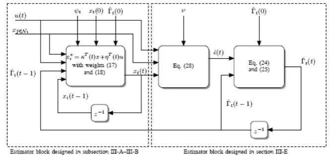
Figure 1: Block diagram of the proposed estimator. It consists of two subsystems in a cascade coupling. The subsystem to the left is an adaptive filter that produces the estimate ofd(t)with small variance and bias. The subsystem to the right is an estimator block that estimates the error covariance matrix
to estimated(t)yield to an over-estimate of the error, which results in poor performance. On the other hand, using onlyx(i)(t)we obtain an under-estimate of the error. This makes the weightsηi(t)rapidly vanish and
the signal measurements are discarded, thus tracking becomes impossible. From these arguments, in order to use bothxi(t)andui(t)we pose a linear least square problem as follows:
min
ˆ
d,βˆ
[ xi ui ] −A [ ˆ d ˆ β ] 2
s.t. ∥B[ dˆ βˆ ]∥2 ≤ρ
withA∈R2Mi×Mi+1andB ∈RMi×Mi+1
A= [
1 I
1 0 ]
, B =[ 0 I ],
andρ being the maxim value of the squared norm of the bias. However, the previous problem is very difficult to solve in a closed form, as it is a Quadratically Constrained Quadratic Problem and it typically requires heavy numerical algorithms to find the solution, such the transformation into aSDPproblem ([55], p. 653). Notice also that, in general, the value ofρis not known in advance, being it a maximum value of the cumulative bias ofMinodes. We thus consider the following regularized problem.
min
ˆ
d,βˆ
[ xi ui ] −A [ ˆ d ˆ β ] 2 +ν B [ ˆ d ˆ β ] 2 (63)
whereν >0is a parameter whose choice is typically rather difficult. The solution of (63) is
( ˆd,βˆ) = [xi, ui]TA[ATA+νBTB]−1.
Proposition 4.4 Ifν >0then
[ATA+νBTB]−1 =
= 1
Mi(1 + 2ν)
[
1 +ν −1T • Mi(1+2ν)I+11T
1+ν
]
(64)
Proof: By Schur’s complement we obtain
[ATA+νBTB]−1 =
(
2Mi−1+Miν
)−1
1T(11T −2Mi(1 +ν)I)−1
• ((1 +ν)I−211MT
i
)−1
From [33], it follows that [
(1 +ν)I−11 T
2Mi
]−1
= I 1 +ν +
11T
Mi(1 + 2ν)(1 +ν) .
It is easy from here to show that the resulting matrix is (64). ∇∇∇
Since we are interested in estimatingϵi(t) =x(t)−d(t)1we observe that such an estimate is given byβˆ.
From the solution of (63), we have ˆ
β= x
i
1 +ν −
ν1Txi(1 +ν)1Tui Mi(1 + 2ν)(1 +ν)
1 (65)
For the choice of the parameterνwe propose to use the Generalized Cross-Validation (GCV) method [34]. This consists in choosing
ν=argmin∥(A
TA+νBTB)−1AT(xi, ui)T∥ T r(ATA+νBTB)−1
Typically the GCV approach is computationally expensive since the trace of the matrix(ATA+νBTB)−1 is difficult to compute, but in our case we have a closed form representation of the matrix, and thus the computation is not difficult. However, it might be computationally difficult to carry out the minimization. Observing that
ν = argmin∥(A
TA+νBTB)−1AT(xi, ui)T∥ tr(ATA+νBTB)−1
≤ argmin∥(A
TA+νBTB)−1AT∥ tr(ATA+νBTB)−1 ∥(x
i, ui)T∥. (66)
a sub-optimal value ofν can be computed solving the right hand side of (66). Notice that the first term in the right hand side of (66) is a function ofν that can be computed off-line and stored in a look-up table at the node. Then, for different data, the problem becomes that of searching in the table.
4.6 Sub-optimal approximation of estimation bias
The previous section explains the estimation of error covariance matrix, which in turn requires computation of two parameters naming, β(t) andν(t). The computation of these parameter causes the increase in the over-all computational complexity of the whole distributed estimation scheme. We propose an alleviation of computingβ(t)by utilizing the fact that in most of the real world data acquisition systems, the contaminating noise lies in frequency bands beyond the signal’s spectrum. Since the data is low-pass filtered prior to estimation, we can assume that most of the noise power has been removed with the application of this filter, and thus (61) can be re-written as
x(i)(t) =d(t)1+ ˜β(t) (67) where
˜
β(t) = ˜βi(t)1
and
˜
βi(t) =uν′i(t)−ui(t)
Though the accuracy ofβ˜iis less thanβˆi, the reduced computational efforts justify this approximation in
the practical estimation systems.
5
Implementation Structure and Numerical Implementation
This section presents the general implementation structure layout of the proposed estimation. Moreover, a figure illustrating the estimator structure and later on the algorithmic implementation is shown followed by some numerical results.
5.1 Layout for the proposed distributed estimation filter design
The general elementary implementation layout showing the connection between different steps can be de-scribed in Table 1 where the first step is involved towards initial conditions for the time delay, the second step defines the steps for the implementation for the FIR low pass filter. The third step shows the estimator stability conditions, which is followed by computational complexity completing the layout for the proposed distributed estimation filter design.
5.2 Estimator Structure and Implementation
Fig. 1 summarizes the structure of the estimator implemented in each node. The estimator has a cascade structure with two sub-systems: the one to the left is an adaptive filter that produces the estimate of d; the one to the right computes an estimate of the error covariance matrix Γi. In the following, we discuss
in some detail a pseudo-code implementation of the blocks in the figure. The estimator is presented as algorithm program 5.2. Initially, the distributed computation of the threshold is performed (lines 1-8): nodeiupdates its thresholdψi until a given precisionω¯ is reached. In the computations ofψi, we chose αi,j(i)=|Nj∩Ni|/(Mi−1)andαi,j(j)=|Nj∩Ni|/(Mj−1). This works well in practice becausekiir, ir=
in Section 3, and the bounds on the error variance in Section 4.3, ensure that estimates among nodes have similar performance.
Numerical results show that the while-loop (lines 4-8) converges after about 10-20 iterations. Line 9 and 10 calculate the time delay of nodeiand all of its neighbor nodes based on the knowledge of propagation speed c. Since there is delaying and advancing of the signal is involved, the farthest node is taken as the reference point and the corresponding time delayτiis taken as the starting time of the algorithm (line 11).
The input signal at each node is then delayed or advanced, depending upon its geometrical location relative to the nodei(line 12-16).These delay-adjusted signal are then filtered to remove the higher frequency noise (line 17-18). The estimators for the local mean estimation error and the local covariance matrix are then initialized (lines 19-20). The main loop of the estimator is lines 23-38. Lines 24-29 are related to the left subsystem of Fig. 1.
The optimal weights are computed using Equations (35) and (36) (lines 27-28). Notice that the optimal Lagrangian multiplier ξi is computed using the function bisection which takes as argument the interval
max(0, σ2√Miψi−λmin(Γi(t−1)))where the optimal value lays. Notice that, if the nodes have limited
computational power, so that the minimum eigenvalue of the matrixΓi(t−1)cannot be exactly computed,
an upper-bound based on Gershgorin’s theorem can be used instead. The estimate ofd(t)is computed in line 29. Lines 30-38 are related to the right subsystem of Figure 1. These lines implement the error covariance estimation by solving the constrained least-squares minimization problem described in subsection 4.5 and 4.6. Sample mean and covariance of the estimation error are updated in lines 36-37. These formulas correspond to recursive implementation of (59) and (60). As an optionβ˜i(t)can be computed using 68.
With regards to the inversions of the estimated error covariance matrixΓˆiin lines 27-28. In general, the
dimension ofΓˆiis not a problem because we consider cases when the number of neighbors is small.
Precau-tions have still to be taken, because even though the error covariance matrixΓiis always positive definite,
its estimateΓˆi may not be positive definite before sufficient statistics are collected. In our implementation,
we use heuristics to ensure thatΓˆiis positive definite.
5.3 Simulation Results
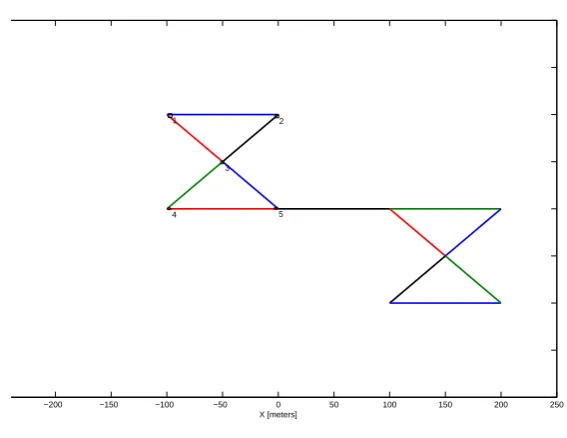
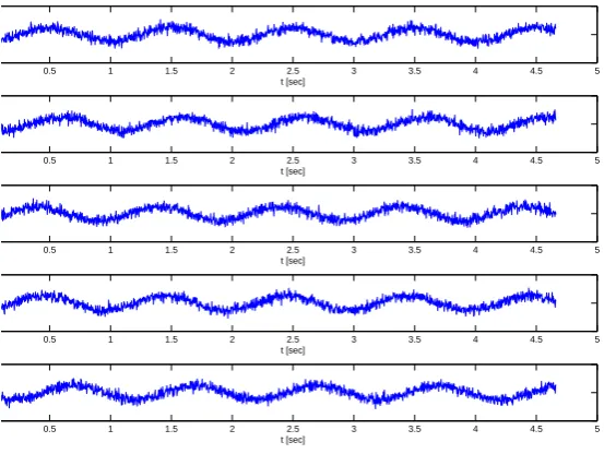
This section shows the simulation results of the proposed filter. Numerical simulations have been carried out in order to validate performance of the proposed distributed estimator. We have simulated a scenario ofN = 10 nodes, with the structure of the sensor network shown in the Fig. 2, where each vertex is the location of a node. Fig. 3 shows the original data d(t), and input datau(τi,vi′)(t) atuτ1,v1′(t)is presented
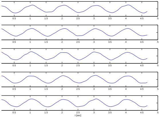
from node1to5, and node6to10in Fig. 4 and 5 respectively. Figs. 6 and 7 show the estimationsx1tox10
for nodes1to10. The data generation from the sensor networks goes through several steps as proposed in the algorithm which during simulation also involves signal generation from all the10nodes, FIR filtering, phase shift calculations and finally the estimation from node1to node10. It has been that how the estimates have been improved by proposed filter algorithm weights, such that the variance of the estimation errors is minimized, thereby improving the estimation results. Moreover, in Fig. 8 and Fig. 9, it has been shown the comparison of the d(t)with its estimate at a specific node 6and10, thus showing the effectivenss of the proposed filter.
6
Conclusion and Future Work
Program 5.2.0.1Estimation algorithm for nodei
STATE t:= 0
ψi(t−1) = 0 ψi(t) = 1/Mi
|ψi(t)−ψi(t−1)| ≥ω¯ = 10−10 ψi(t+ 1) =Ti(ψ(t))
Collect thresholds from nodes inΘi t:=t+ 1
ENDWHILE STATE τi = rci
τj = rcj, j ∈Mi τj = rcj, j ∈Mi
t:=max(τi), i= 1,2,3, ..., N
IF rj < ri uv′
j(t) =u(τj,vj′)(t−τj)
ELSE IFri < rj uv′
j)(t) =u(τj,v′j)(t+τj)
END
STATEui(t) =F ilter(uvi′)(t))
ui(t) =F ilter(uv′i)(t))
uj(t) =F ilter(uvj′)(t)), j∈Mi t:=max(τi), i= 1,2,3, ..., N
ˆ
mei(t) := 0
ˆ
Γi(t) :=σ2I xi(t) :=ui(t)
WHILE FOREVER STATEMi :=|Ni|
t:=t+ 1
ξi = bisection(max[0, σ2/
√
Miψi−λmin(Γi(t−1))]) κi(t) := σ
2(ˆΓ
i(t−1)+ξiI)−11
Mi+σ21T(ˆΓi(t−1)+ξiI)−11
ηi(t) := M 1
i+σ21T(ˆΓi(t−1)+ξiI)−11
xi(t) :=
∑
j∈Niκijxj(t−1) +
∑
j∈Niηij(t)uj(t)
ˆ
β := 1+xiν −ν1MTxi+(1+ν)1Tui
i(1+2ν)(1+ν) 1
OR ˜
βi(t) :=uνi′(t)−ui(t)
ˆ
ϵi := ˆβ
OR ˆ
ϵi := ˜β
ˆ
mei(t) :=
t−1
t mˆei(t−1) +
1
tˆϵi(t)
ˆ
Γi(t) := t−t1Γˆi(t−1) +1t(ˆϵi(t)−mˆei(t))(ˆϵi(t)−mˆei(t))
T
..
−200 −150 −100 −50 0 50 100 150 200 250 X [meters]
2
4 5
3 1
Figure 2:Structure of Sensor network. Note that, for example, node 1 has node 2 and node 3 as neighbors, while node 3 has node 1, node 2, node 4, and node 5 as neighbors.
..
0.5 1 1.5 2 2.5 3 3.5 4 4.5 5
t [sec]
0.5 1 1.5 2 2.5 3 3.5 4 4.5 5
t [sec]
0.5 1 1.5 2 2.5 3 3.5 4 4.5 5
t [sec]
0.5 1 1.5 2 2.5 3 3.5 4 4.5 5
t [sec]
0.5 1 1.5 2 2.5 3 3.5 4 4.5 5
t [sec]
..
0.5 1 1.5 2 2.5 3 3.5 4 4.5 5
t [sec]
0.5 1 1.5 2 2.5 3 3.5 4 4.5 5
t [sec]
0.5 1 1.5 2 2.5 3 3.5 4 4.5 5
t [sec]
0.5 1 1.5 2 2.5 3 3.5 4 4.5 5
t [sec]
0.5 1 1.5 2 2.5 3 3.5 4 4.5 5
t [sec]
Figure 4:The inputuτi,v′
i(t)at node i, for i=1,2,... 5
..
0.5 1 1.5 2 2.5 3 3.5 4 4.5 5
t [sec]
0.5 1 1.5 2 2.5 3 3.5 4 4.5 5
t [sec]
0.5 1 1.5 2 2.5 3 3.5 4 4.5 5
t [sec]
0.5 1 1.5 2 2.5 3 3.5 4 4.5 5
t [sec]
0.5 1 1.5 2 2.5 3 3.5 4 4.5 5
t [sec]
..
0.5 1 1.5 2 2.5 3 3.5 4 4.5 5
0.5 1 1.5 2 2.5 3 3.5 4 4.5 5
0.5 1 1.5 2 2.5 3 3.5 4 4.5 5
0.5 1 1.5 2 2.5 3 3.5 4 4.5 5
0.5 1 1.5 2 2.5 3 3.5 4 4.5 5
t [sec]
Figure 6: Estimates ofd(t)at node 1 to node 5
..
0.5 1 1.5 2 2.5 3 3.5 4 4.5 5
0.5 1 1.5 2 2.5 3 3.5 4 4.5 5
0.5 1 1.5 2 2.5 3 3.5 4 4.5 5
0.5 1 1.5 2 2.5 3 3.5 4 4.5 5
0.5 1 1.5 2 2.5 3 3.5 4 4.5 5
t [sec]
..
0 500 1000 1500 2000 2500
−3 −2 −1 0 1 2 3
Number of Observations
original data estimate at node 6
Figure 8: Comparison ofd(t)and estimatedd(t)at node 6
..
0 500 1000 1500 2000 2500
−3 −2 −1 0 1 2 3
Number of Observations
original data estimate at node 10