e-ISSN: 2278-067X, p-ISSN: 2278-800X, www.ijerd.com
Volume 9, Issue 11 (February 2014), PP. 15-23
Economic Load Dispatch Solution Including Transmission
Losses Using MOPSO
1
G. Sarath Babu,
2S.Anupama,
3P.Suresh babu
1PG Student, Annamacharya Institute of Technology & Sciences, Rajampet
2Assistant Professor, Department of EEE, Annamacharya Institute of Technology & Sciences, 3
Mr. P. Suresh Babu, Assistant Professor, Department of EEE, Annamacharya Institute of Technology & Sciences, Rajampet
Abstract:- Economic Dispatch is an important task in power system. It is the process of allocating generation among the committed units such that the constraints imposed are satisfied and the energy requirements are minimized. This paper presents efficient approach for Dynamic Economic Load Dispatch (DELD) solution with transmission losses based on Multi Objective Particle Swarm Optimization (MOPSO). The main objective is to determine the most economic dispatch of on line generating units with the predicted load demands over a certain period of time.The proposed algorithm evaluates a set of Pareto solutions systematically and preserves the diversity of Pareto by crowding entropy diversity. The crowding entropy strategy is able to measure the crowding degree of the solutions more accurately and efficiently. Here, an attempt is made to find the minimum cost using MOPSO method for 6 and 15 unit test systems with continuous demands for 24 hours. The effectiveness and feasibility of the proposed method is demonstrated in this paper. The MATLAB results are compared with the recent reports using Brent method in terms of solution quality. Numerical results indicate an improvement in total fuel cost saving and hence the superiority of the proposed is also revealed for dynamic economic dispatch problems.
Keywords:- MOPSO, Dynamic Economic Load Dispatch, Pareto Optimal Solution, Transmission Loss.
I.
INTRODUCTION
Power systems should be operated under a high degree of economy for competition of deregulation. Unit commitment is an important optimization task addressing this crucial concern for power system operations. Since Economic Dispatch (ED) is the fundamental issue during unit commitment process, it should be important to obtain a higher quality solution from ED efficiently. The primary objective of the economic dispatch problem is to schedule the generations of the online thermal units so as to meet the required load demand at minimum operating cost while satisfying the unit and system equality and inequality constraints. Dynamic Economic Dispatch (DED) is an extension of the economic dispatch problem and it aims to schedule the online thermal units with the predicted load demands over a scheduling period at minimum operating cost. DED problem is formulated as minimization of total fuel cost is the main objective while satisfying system constraints. The DED problem has been formulated as a second order quadratic optimization problem that takes into the consideration of the ramp rate limits of the generating units [1-2].
comparison with the performance of Brent method [5]. The results evaluation reveals that the proposed MOPSO algorithm achieves good quality solution for DED problem and is superior to the Brent method one.
II.
PROBLEM FORMULATION
The DED problem is formulated as the minimization of total fuel cost of generating units for the entire scheduling period subject to variety of constraints. The DED problem formulation is as follows.
A. Objective function
The main objective of DED problem is to minimize the generation cost of „n‟ online thermal units over a scheduling period „T‟ is given as,
min 𝑇𝑡=1 𝑁𝑖=1𝐹𝐶𝑖(𝑃𝑡𝑖) … (1)
Where, FCi,t is the fuel cost of unit i at time interval t in $/h and Pi,t is the real power output of generating unit i at time period t in MW.
The fuel cost (FC) of generating unit at any time interval„t‟ is normally expressed as a quadratic function is as,
𝐹𝑖 𝑃𝑡𝑖 = 𝑎𝑖+ 𝑏𝑖𝑃𝑖+ 𝑐𝑖𝑃𝑖2 … (2) Where, ai, bi and ci are the cost coefficients of generating unit i.
B. Constraints
The objective function is minimized subject to variety of constraints.
1) Power balance constraint
This constraint is based on the principle of equilibrium that the total generation at any time interval „t‟ should satisfy the load demand at the interval „t‟ and transmission loss. This constraint is mathematically expressed as,
𝑃𝑖= 𝑃𝐷+ 𝑃𝐿 𝑛
𝑖=1
… (3)
Where, PD,t and PL,t are the load demand and transmission loss in MW at time interval „t‟ respectively.
The transmission loss can be expressed using through B coefficients.
𝑃𝐿= 𝑃𝑖𝐵𝑖𝑗𝑃𝑗 𝑛 𝑗 =1 + 𝑛 𝑖=1
𝐵0𝑖𝑃𝑖+ 𝐵00 𝑛
𝑖=1
… (4)
Where, Bij, B0i and B00 are the loss coefficients.
2) Generator operational constraints
The generating unit operational constraints such as minimum/maximum generation limit, ramp rate limits and prohibited operating zones are as follows.
a) Generator capacity constraint
Pi,min< 𝑃𝑖< 𝑃𝑖,𝑚𝑎𝑥 … 5
Where, Pi,min and Pi,max are the minimum and maximum real power generation of unit i in MW.
b) Ramp rate limits
The inequality constraints due to ramp rate limits for unit generation changes are given 1) as generation increases
𝑃𝑖 − 𝑃𝑖0≤ 𝑈𝑅𝑖 … (6) 2) as generation decreases
𝑃𝑖 − 𝑃𝑖0≤ 𝐷𝑅𝑖 … (7)
The generator operation constraint after including ramp rate limit of generators can be described as, max(Pi,min, 𝑃𝑖0 - DRi)< 𝑃𝑖 < min(Pi,max, 𝑃𝑖0 + URi) …(8)
where, 𝑃𝑖0, DRi and URi are the real power output of generator i before dispatched hour in MW, down
ramp and up ramp limit of generator i in MW/h respectively.
III.
MULTI OBJECTIVE PARTICLE SWARM OPTIMIZATION
3.1. PSO Overview
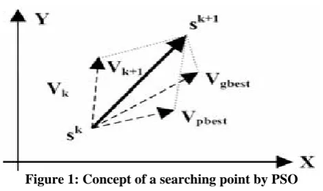
Figure 1: Concept of a searching point by PSO
This modification can be represented by the concept of velocity. Velocity of each agent can be modified by the following equation:
vidk+1= ωvidk+ c1 rand* pbestid- sid k +
c2 rand* gbestd- sidk (9)
Using the above equation, a certain velocity, which gradually gets close to pbest and gbest can be calculated. The current position (searching point in the solution space) can be modified by the following equation:
sidk+1= sidk+ vidk+1 (10)
where sk is current searching point, sk+1 is modified searching point, vkis current velocity, vk+1is modified velocity of agent i, vpbest is velocity based on pbest, , vgbest is velocity based on gbest, n is number of particles in a
group, m is number of members in a particle, pbesti is pbest of agent i, gbesti is gbest of the group, ωi is weight
function for velocity of agent i, Ci is weight coefficients for each term. Appropriate value ranges for C1 and C2
are 1 to 2, ωi is taken as 1.
3.2 MULTI OBJECTIVE PSO (MOPSO)
A lot of realistic life problems entail simultaneous optimization of some objective functions. In general, these functions are non-commensurable and often competing and conflicting objectives. The application of a multi objective optimizer makes it possible to envisage the trade off among different conflicting objectives to direct the engineer in making his compromise and gives rise to a set of optimal solutions, in place of one optimal solution. The concept of Pareto dominance formulated by Vilfredo Pareto is used for the evaluation of the solutions [7].
The solutions that are nondominated within the whole search space are signified as Pareto-optimal and constitute the Pareto-optimal set. This set is also known as Pareto optimal front. Pareto dominance concept classifies solutions as dominated or non-dominated solutions and the “best solutions” are selected from the
non-dominated solutions. The implemented algorithm is the non-non-dominated sorting PSO which is currently used in many other practical design problems. To sort non-dominated solutions, the first front of the non-dominated solution is assigned the highest rank and the last one is assigned the lowest rank. When comparing solutions that belong to a same front, another parameter called crowding distance [17] is calculated for each solution. The crowding distance is a measure of how close an individual is to its neighbours.
Large average crowding distance will result in better diversity in the population. In order to investigate multi-objective problems, some modifications in the PSO algorithm were made. A multiobjective optimization algorithm must achieve: guide the search towards the global Pareto-optimal front and maintain solution diversity in the Pareto-Optimal front. The main steps of the MOPSO algorithm for DED problem are explained in more detail as follows:
Step 1: Input parameters of system, and specify the lower and upper boundaries of each variable.
Step 2: Initialize randomly the speed and position of each particle and maintain the particles within the search space.
Step 3: For each particle of the population, employ the Newton-Raphson power flow analysis method to calculate power flow and system transmission loss, and evaluate each of the particles in the population.
Step 4: Store the positions of the particles that represent non-dominated vectors in the repository NOD.
Step 5: Generate hypercubes of the search space explored so far, and locate the particles using these hypercubes as a coordinate system where each particle‟s coordinates are defined according to the values of its objective function.
Step 6: Initialize the memory of each particle in which a single local best for each particle is contained.
Step 7: Update the time counter t=t+1.
number x>1 by the number of particles that they contain. Then, we apply crowding distance method using these fitness values to select the hypercube from which we will
take the corresponding particle. Once the hypercube has been selected, we select randomly a particle as the best global particle Gbest for particle i within such hypercube.
Step 9: Compute the speed and its new position of each particle using Equations (12) and (13), and maintain the particles within the search space in case they go beyond its boundaries.
Step 10: Evaluate each particle in the population by the Newton-Raphson power flow analysis method.
Step 11: Update the contents of the repository NOD together with the geographical representation of the particles within the hypercubes.
Step 12: Update the contents of the repository Pbest.
Step 13: If the maximum iterations itermax are satisfied then go to Step 14,otherwise, go to step7.
Step 14: Input a set of the Pareto-optimal solutions from the repository NOD.
3.3. Non-Dominated Sort
The initialized population is sorted based on nondomination. The fast sort algorithm as given in [8] is used here for NOD.
3.4. Crowding Distance
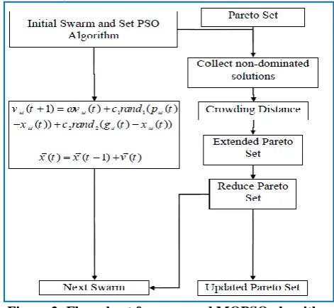
Once the non-dominated sort is complete, the crowding distance is assigned. As the individuals are selected based on rank and crowding distance all the individuals in the swarm are assigned a crowding distance value. Crowding distance is allocated front wise and comparing the crowding distance between two individuals in different front is meaningless. The algorithm as given in [8] is used here for the crowding distance. The flowchart of the proposed MOPSO algorithm is shown in Figure 2.
Figure 2: Flow chart for proposed MOPSO algorithm
IV.
RESULTS AND DISCUSSIONS
The proposed methodology for solving DED problem is implemented in Matlab 7.8 platform and executed with personal computer. The effectiveness of the proposed methodology has been tested with two different scales of power system cases. The six unit and fifteen unit system are considered for the analysis. The generating unit operational constraint, ramp rate limits and transmission loss are considered. The results obtained from the proposed method were compared in terms of the solution quality and computation efficiency with the Brent method [9]. In each test system, 30 independent runs were made for each of the optimization methods.
Case 1: Six unit system
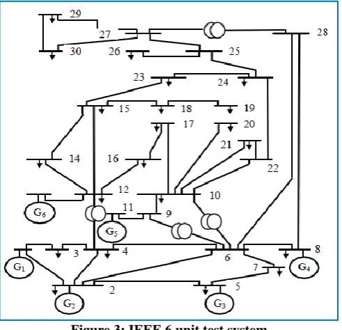
electrical network on IEEE 30 bus including six thermal generating units as shown in Figure 3 to assess the suitability of the algorithm. The fuel cost (in $/hr), ramp rate limits and data of predicted power demands is extracted from [11] are given in Tables 1-3, respectively.
Figure 3: IEEE 6 unit test system
Table 1: Fuel cost of six units system
U ai ($) bi ($/MW) ci ($/MW2) Pimin (MW) Pimax
1 240 7 0.007 100 500
2 200 10 0.0095 50 200
3 220 8.5 0.009 80 300
4 200 11 0.009 50 150
5 220 10.5 0.008 50 200
6 190 12 0.0075 50 120
Table 2: Ramp rate limits of six units system Unit Pi0 (MW) URi (MW/h) DRi (MW/h)
1 340 80 120
2 134 50 90
3 240 65 100
4 90 50 90
5 110 50 90
6 52 50 90
Table 3: Predicted power demand of six units in 24 hours
H 1 2 3 4 5 6 7 8
PD (MW) 955 942 935 930 935 963 989 102.3
H 9 10 11 12 13 14 15 16
PD (MW) 112 6115 120 1123 5119 125 1126 3125
H 17 18 19 20 21 22 23 24
PD (MW) 122 1120 2115 9109 2102.3 984 975 960
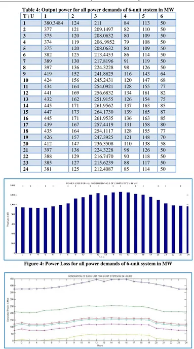
Table 4: Output power for all power demands of 6-unit system in MW
T \ U 1 2 3 4 5 6
1 380.3484 124 211 84 113 50
2 377 121 209.1497 82 110 50
3 375 120 208.0632 80 109 50
4 374 119 206..9952 79 108 50
5 375 120 208.0632 80 109 50
6 382 125 213.4453 86 114 50
7 389 130 217.8196 91 119 50
8 397 136 224.3228 98 126 50
9 419 152 241.8625 116 143 64
10 424 156 245.2431 120 147 68
11 434 164 254.0921 128 155 77
12 441 169 256.6832 134 161 82
13 432 162 251.9155 126 154 75
14 445 171 261.9562 137 163 85
15 447 173 264.1730 139 165 87
16 445 171 261.9535 136 163 85
17 439 167 257.4419 131 158 80
18 435 164 254.1117 128 155 77
19 426 157 247.3925 121 148 70
20 412 147 236.3508 110 138 58
21 397 136 224.3228 98 126 50
22 388 129 216.7470 90 118 50
23 385 127 215.6239 88 117 50
24 381 125 212.4087 85 114 50
Figure 4: Power Loss for all power demands of 6-unit system in MW
Case 2: Fifteen unit system
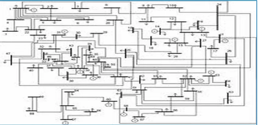
The system contains 15 thermal units and the details including cost coefficients, generation limits, ramp rate limits, transmission loss coefficients and forecasted load demand of each interval are presented in the literature [12]. The transmission loss is calculated using B coefficients. The one day scheduling period is divided into 24 intervals. The optimal dispatch of generating units is determined by MOPSO. The minimum and maximum operating limit of each generating unit is obtained by enforcing the ramp down and ramp up limits of generating unit with the real power dispatch of previous interval. The proposed method is applied to the electrical network on IEEE 69 bus including 15 thermal generating units as shown in Figure 6 to assess the suitability of the algorithm.
Figure 6: IEEE 69 bus system with 15 thermal generating units
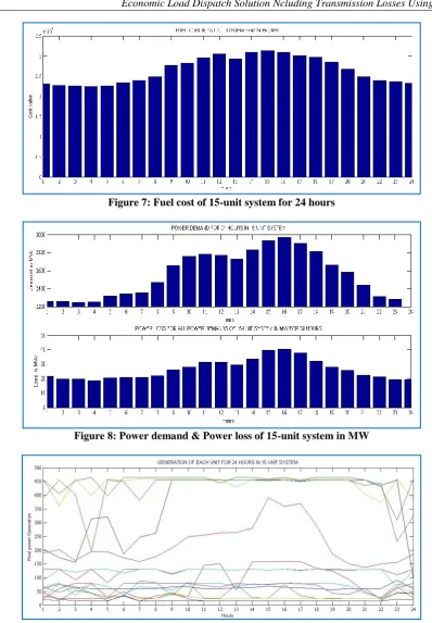
Table 5 and figure 7 represents the optimal output powers and power loss for all power demands using the proposed MOPSO method and also it is clear that this technique provides better solutions for DED problem compared with the other reported methods in the paper. Figure 8 represents the fuel cost for the 15-unit system and Figure 9 represents the generation of each unit in 15 unit test system for 24hours.
Table 5: Output power for all power demands of 15-unit system in MW
H OUTPUT POWER IN MW LOSS
MW
P1 P2 P3 P4 P5 P6 P7 P8 P9 P10 P11 P12 P13 P14 P15
1 204.43 388.14 130 90.96 190.56 460 454.37 60 66.01 33.71 66.74 21.16 25 20.44 46.15 21.6640
2 172.45 455 130 130 202.6 361.28 406.86 76.11 47.08 25 80 60.35 77 16.94 19.42 19.7916
3 155.32 402.06 91.55 120.52 162.68 460 452.56 65.56 65.09 25 36.62 80 58.14 53.17 17.51 19.5049
4 313.71 196.95 130 130 195.49 395.55 465 60 43.43 25 80 80 76.07 44.87 15.07 18.8160
5 322.28 455 82.35 130 193.91 460 397.14 60 30.44 25 68.62 27.81 34.97 16.30 15.04 20.5173
6 185.72 449.02 130 116.93 173.32 453.32 465 60 34.23 48.05 40.61 80 31.64 33.24 36.31 21.0411
7 246.93 381.80 130 130 158.21 460 465 60 88.46 26.52 67.02 80 28.08 15.22 15 20.9092
8 261.95 455 130 130 177.51 460 465 60 83.43 25.02 63.73 80 25 34.13 15.86 22.1049
9 455 455 114.44 112.68 207.20 460 465 67.36 35.76 40.60 55.34 80 46.83 44 17.10 26.3608
10 455 455 130 130 248.08 460 465 67.46 84.45 31.01 80 80 31.32 22.89 16.84 28.0837
11 455 455 130 130 254.67 460 465 60 25.34 145.2 80 70.34 25 15 15 31.1440
12 455 455 129.94 129.26 262.74 457.85 444.69 60.1 25.25 150.15 80.63 65.07 25.01 15.01 15.03 31.2921
13 455 455 127.73 128.32 265.11 429.34 465 63.31 76.49 55.31 68.77 80 25.63 15.94 16.23 29.2897
14 455 455 130 130 280.85 457.04 465 64.81 26.93 157.60 77.81 75.07 25 15 15 33.4710
15 455 452.64 128.03 127.40 390 460 458.91 70 25.70 157.88 75.05 75.72 26.32 15.22 15.78 39.3182
16 455 455 130 130 360.23 460 465 65 75.53 160 80 80 25.95 15 15.20 40.4463
17 455 451.29 128.07 126.44 370 455 455.55 62.80 35.15 158.22 76.98 78.27 25.06 15.16 15.57 37.9225
18 450 455 130 130 290.23 457.76 465 60 25 134.23 80 73.19 25 15 15 32.3263
19 455 455 128.97 130 185.43 460 465 56.44 25 123.56 80 43.54 25.54 15.78 15.01 28.0054
20 454.43 454.87 127.98 128.99 150 460 465 60 25 93.54 69.56 38.65 25 15 15 25.6883
21 455 435.43 129.76 129.90 136.98 404.32 455 60 25 49.34 44.76 61.54 25 15 15 22.5091
22 435.65 445 130 130 150 373.76 430 60 25 25.21 27.76 20 25 15 15 21.2422
23 455 231.98 111 68.42 156.32 460 309.33 9321.29 42.96 66.96 77.35 62.23 77.36 47.70 22.45 19.4106
Figure 7: Fuel cost of 15-unit system for 24 hours
Figure 8: Power demand & Power loss of 15-unit system in MW
Figure 9: Generation of each unit for 24 hours in 15-unit system
V.
CONCLUSION
REFERENCES
[1]. X.S. Han, H. B. Gooi, and D. S. Kirschen, “Dynamic economic dispatch: Feasible and optimal solutions”, IEEE Trans. Power Systems, vol. 16, no. 1, pp. 22-28, Feb. 2001.
[2]. W.R. Barcelo and P. Rastgoufard, “Dynamic dispatch using the extended security constrained economic dispatch algorithm”, IEEE Trans. Power Systems, vol. 12, no. 2, pp. 961-967, May 1997. [3]. B.K. Panigrahi, V. Ravikumar Pandi, D. Sanjoy, “Adaptive Particle Swarm Optimization Approach for
Static and Dynamic Economic Load Dispatch”, Energy Conversion and Management, Vol. 49, pp. 1407-1415, 2008.
[4]. D.W. Ross, S. Kim, “Dynamic Economic Dispatch of Generation”, IEEE Trans. on Power Apparatus Systems, Vol. 99, No. 6, pp. 2060-7, 2002.
[5]. C.K. Panigrahi, P.K. Chattopadhyay, R. Chakrabarti, “Load Dispatch and PSO Algorithm for DED Control”, International Journal of Automation and Control, Vol. 1, pp 195- 206, 2007.
[6]. Kennedy J and Eberhart R, “Particle Swarm Optimizer,” IEEE International Conference on Neural Networks (Perth, Australia), IEEE Service Center Piscataway, NJ, IV, pp1942- 1948, 1995.
[7]. P.Phonrattanasak, “Optimal placement of DG using multiobjective particle swarm optimization”,
Proceedings of International conference on Mechanical and Electrical Technology, ICMET-2010, Thailand.
[8]. K. Deb, A. Pratap, S. Agarwal, T. Meyarivan, “A Fast and Elitist Multi-Objective Genetic Algorithm: NSGA-II”, IEEE Trans. on Evolutionary Computation, Vol. 6, No. 2, pp. 182-197, 2002.
[9]. K. Chandram, N. Subrahmanyam, M. Sydulu, “Brent Method for Dynamic Economic Dispatch with Transmission Losses”, Iranian Journal of Electrical and Computer Engineering, Vol. 8, No. 1, pp. 16-22, 2009.
[10]. J. Wood and B.F. Wollenberg, “Power Generation”, Operation, and Control, 2nd Ed. New York: Wiley, 1996.
[11]. H. Saadat, “Power System Analysis”, McGraw-Hill, New York, 1999.
[12]. B.H. Chowdhury, S. Rahman, “A Review of Recent Advances in Economic Dispatch”, IEEE Trans. on Power Systems, Vol. 5, No. 4, pp. 1248-1259, 1990.
[13]. B. Balamurugan, R. Subramanian, “Differential Evolution Based Dynamic Economic Dispatch of Generating Units with Valve Point Effects”, Electric Power Components Systems, Vol. 36, pp. 828-843, 2008.