RESEARCH ARTICLE
SIMULATION OF THE IONOSPHERIC EFFECT OF INTENSE GEOMAGNETIC STORMS OF
JULY AND NOVEMBER 2004 USING A LOW LATITUDE 3D THEORETICAL MODEL
*
Dr. Arup Borgohain
North Eastern Space Applications Centre, Dept. of Space, Govt. of India,
Umiam-793103, Meghalaya, India
ARTICLE INFO ABSTRACT
The performance of the Dibrugarh University low latitude 3D theoretical model at different geomagnetic activity levels and for intense geomagnetic storms has been investigated. In this model the continuity, momentum and energy balance equations of ion and electron flux along geomagnetic field lines from the Northern to the Southern hemisphere are solved simultaneously. The model is used to simulate electron density at different geomagnetic activity conditions Ap=5, 10, 20. With the increase of the geomagnetic activity, the Equatorial Ionization Anomaly (EIA) exhibits a tendency to come closure towards low latitudes and the EIA merges at Ap=20. The effect of two intense geomagnetic storms that occurred in July & November 2004 on Total Electron Content (TEC) has been investigated and compared with observed TEC data. Agreement between model and measured data was found to be very good.
INTRODUCTION
A geomagnetic storm is the result of strong enhancement of ring currents in which the earth’s magnetic field is usually depressed below its quiet day value. Solar wind energy captured by the magnetosphere may induce influences of different magnitude on the complex morphology of the electric fields, temperature, winds and composition and affect all ionospheric parameters. One of the main characteristics of the disturbed ionosphere is a great degree of variability. Due to the interaction of many different factors, each storm shows a different course. The F2 region response to a geomagnetic storm is known as an ionospheric storm. Ionospheric storms represent an extreme form of space weather, which can have a significant adverse effects on increasingly sophisticated ground and space based technological systems of our society. The ionospheric effects are dependent on the time of storm occurrence and intensity, as well as on the latitude of the station and its location in the summer or in the winter hemisphere. The local time or longitude dependent response of storm time irregularities often shows substantial differences in irregularity activity at nearby longitude regions (Basu et al., 2001a; Sahai et al., 2005; Sreeja et al., 2009). Both the prompt equatorward penetration of magnetospheric or high-latitude electric fields and the ionospheric disturbance dynamo significantly alter the ionospheric electric fields in the equatorial and low-latitude regions (Fejer and Scherliess, 1997).
*Corresponding author: Dr. Arup Borgohain,
North Eastern Space Applications Centre, Dept. of Space, Govt. of India, Umiam-793103, Meghalaya, India.
Basu et al., (2001) illustrated the response of the equatorial ionosphere in the South Atlantic region to the great geomagnetic storm of July 15, 2000 studied by ground based TEC and satellite in situ measurements (DMSP and FORMOSAT-1). Responses of equatorial anomaly to the October–November 2003 super storms reported by Zhao et al. (2005) using the total electron content (TEC) measured with global positioning system (GPS) receivers in China, Southeast Asia, Australian (CSAA), and the American regions. Theoretical study of new plasma structures in the low-latitude ionosphere during a major magnetic storm has been done by Lin et al (2009). Guozhu et al., (2010) reported the longitudinal development of low-latitude ionospheric irregularities during the geomagnetic storms of July 2004. They found that the irregularities occurred over a wide longitudinal range, extending from around 300°E to 120°E on storm days 25 and 27 July 2004.Li et al. (2009) characterizing the 10th November 2004 storm time middle latitude plasma bubble event in Southeast Asia using multi instrument observations. Rama Rao et al., (2009) reported the variation of the total electron content (TEC) from 6th to 11th November 2004 measured at seven different stations in the Indian sector which are set along a common meridian of 77º E and covering the equatorial to the anomaly crest regions and beyond during the geomagnetic storms of 8th to 10th November 2004. Bagiya et al. (2015) studied the ionospheric response in the Indian sector during the prolonged geomagnetic storm of July 2012. Recently, Kalita et al. (2016) studied the response of the March 17 2013 and 2015 storms on TEC and NmF2 in a meridional chain of stations along 100°E.
Article History:
Received 24th January, 2017
Received in revised form 18th February, 2017
Accepted 05th March, 2017
Published online 30th April, 2017
International Journal of Recent Advances in Multidisciplinary Research
Vol. 04, Issue 04, pp.2512-2518, April, 2017
Keywords:
The theoretical model and TEC data
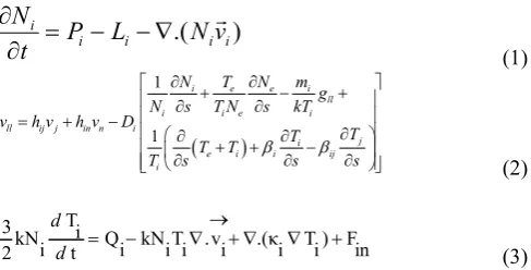
In this study the Dibrugarh University low latitude 3D theoretical density and temperature model for the Indian longitudinal sector developed by Bhuyan et al. (2007) is used. In this model the continuity (eq. 1), momentum (eq. 2) and energy balance (eq. 3) equation of ion and electron flux are simultaneously solved along geomagnetic field lines from the northern to the southern hemisphere. The effects of E × B drift, horizontal wind, magnetic field, solar activity and chemical reactions are considered for the calculation of density. Heating due to photoelectrons, collision between ions, ions and electrons, rotational heat transfer, vibrational heat transfer and thermal conductivity are considered for calculation of electron and ion temperatures.
The following equations are solved simultaneously.
)
.(
i ii i
i
P
L
N
v
t
N
(1) (2) (3)
Here, N is the ion density, P and L are the ion production and ion loss rates respectively and V is the ion transport velocity. The momentum equation for the ith ion, as given by Moffett et al. (1989) gives the form of the field-aligned ion velocity used in the model. Equation (3) represents the energy balance equation for the ith constituent (where i=O+, H+, or e). where Qi
gives heating rate (positive or negative) due to collisional interactions with other ion or neutral species, the second and third terms on the right hand side are due to adiabatic heating/cooling and thermal conductivity respectively. κi (eVm
–1
s-1K-1) is the thermal conductivity for ith ion as given by Banks and Kockarts (1973).The thermal conductivity κe for
electrons is given by Schunk and Nagy (1978). Fin is the
frictional heating due to the relative motion between the ith ion and neutral gases. The production of O+ is assumed due to both photo ionization and chemical process. The production of H+ is considered only due to the resonant charge exchange reaction with oxygen (Stubbe, 1970). The chemical reaction rates are as given by Raitt et al. (1975) whereas the rate coefficients for loss of O+ following charge exchange reactions with O2 and N2
are taken from Torr and Torr (1979).
Initially the sensitivity of the model at different geomagnetic activity conditions is examined. So with the provision for different input parameters, model code was tuned for different Ap indices and F10.7. The model outputs are then compared with the Total Electron Content (TEC) data obtained by GPS receivers. The electron density (m-3) simulated across the geomagnetic field lines is vertically integrated to get TEC (m-2) using the Runge Kutta numerical integration method. GPS slant TEC (STEC) measurements were made simultaneously at eighteen locations in India since April 2004 using identical dual frequency GPS receivers under the project GAGAN (Geo And
GPS Augmented Navigation). Coordinates of these eighteen stations, separated in latitude and longitude by ~5º across India. In this study TEC over Ahmedabad (14.7ºN, 146.3ºE), at the crest of the EIA and Trivandum (0.3ºS, 149.2ºE) at the magnetic equator has been considered. STEC is converted to vertical TEC using a suitable mapping function.
RESULTS
Response of the model for different levels of geomagnetic activity
Enhancement of the solar wind and CMEs during geomagnetic storms manifests in the geomagnetic field as well as the electrodynamics of ionosphere. During magnetically disturbed conditions, the low latitude electric field and current undergoes large departures from their quiet day average (Fejer, 1986; Abdu, 1995). The disturbance level can be gauged by the proxy planetary index Ap. The enhanced solar wind during disturbed time on arrival at the boundary of magnetosphere increases the compression of the magnetic field and a modification of magnetic field as well as the electric field. During magnetically active conditions, the disturbance electric field and dynamo action of disturbance winds are driven by enhanced energy and momentum deposition into the high latitude ionosphere by Joule heating and particle precipitation (Blanc and Richmond 1980).The disturbance dynamo drives a downward plasma drift during the day and upward at night opposite to the quiet day field (Fuller, 2002).
So the electron density distribution changes due to the damping of the normal diurnal variation in vertical drift. These storm-time changes in thermospheric compositions and ionospheric electron densities affect electron temperature (Wang, 2006). In addition to the inverse dependence of electron temperature on electron density, electron temperature is also controlled by the disturbed time strong meridional winds and electric field. In this study, model inputs have been fitted for solar minimum equinoctial conditions with provision for different geomagnetic activity (Ap) levels. Model was run for Ap=5, 10, 20. Model
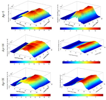
shows good response at different geomagnetic conditions. Figure 1 shows the diurnal plot of electron density at 300 km and 500 km respectively. Results show diurnal minimum ~ 2×10¹¹ m-3 before sunrise (06:00LT) with diurnal maximum ~ 1.6×10¹¹ m-3 in 15:00 LT at ~ 300 km altitude. The diurnal maximum and minimum at 500 km is ~ 2×10¹¹ m-3 and ~ 1.6×10¹¹ m-3 respectively. Good construction of EIA with diurnal maximum 1.6×10¹² m-3 is observed for Ap=5 at ~300 km altitude. With the increase of the geomagnetic activity levels, the EIA has a tendency to come closure towards low latitudes and EIA merges at Ap=20.
Simulation of the intense geomagnetic storms of 2004
Ionospheric F2-region disturbances are produced in association with geomagnetic storms. Such disturbances basically increase or decrease the maximum electron density NmF2 from median or quiet time values. During geomagnetic storms the disturbed solar wind-magnetosphere interactions affect the mid and low latitude F region due to intense transient magnetospheric convective electric field (Sastri et al 1992; Foster and Rich 1998) and neutral wind. The electric field associated with the ring current development and decay manifests as a sharp decrease in DST magnitude, followed by recovery phase.
1
1
i e e i
ll
i i e i
ll ij j in n i
j i
e i i ij
i
N T N m
g
N s T N s kT
v h v h v D
T T
T T
T s s s
The electric fields associated with a disturbance dynamo also appear at low and equatorial latitudes. The E×B drifts associated with the electric fields at low latitudes appear to explain largely daytime ionization redistribution and changes EIA. The meridional neutral winds also play an important role in ionization at low latitudes (Subrahmanyam et al., 2005). The electric field and meridional winds both contribute to the vertical drifts of the ionospheric plasma. The current theoretical model is sensitive enough to the above geomagnetic and wind conditions. Table 1 (Part I & II) shows the Ap indices and solar F10.7 for the consecutive storm days of 22-27th July
2004 and 7- 11th November 2004. The model has been run for the geomagnetic conditions on every day of the geomagnetic storm of July and November 2004. The zonal and meridional wind changes with the conditions.
The model incorporates sufficiently plasma tube to solve the model equations for providing reasonable full diurnal coverage. Also the vertical drift is a function of height. The electron density data generated by the model code are extracted for the two locations Trivandrum (0.3ºS, 149.2ºE, geomagnetic) and Ahmedabad (14.7ºN, 146.3ºE, geomagnetic), where GPS measured TEC data are available. The data have been integrated vertically at the observation point and the total columnar electron density i.e. TEC value calculated.
Over Ahmedabad (14.7ºN, 146.3ºE)
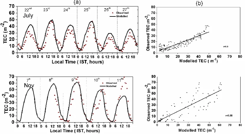
The modelled TEC values are compared with the observed TEC value over Ahmedabad. Figure 3a (top) shows day-to-day variation of TEC measured by GPS network and TEC derived
Figure 1. Simulated Electron Density in different geomagnetic activity levels (Ap=5,10, 20) at 300km (left) and 500km (right) altitude
Table 1. Day to day variations of Ap indices and F10.7 during the storm period 22-27th July 2004.
Part I Storm period: 22-27th July 2004. Part II Storm period: 7-11th November 2004
Date Day No Ap F10.7 Monthly Average Date Day No Ap F10.7 Monthly Average
22nd 204 31 172
Ap=22.8 F10.7=18.5
07th 312 50 129
Ap=25 F10.7=113
23rd 205 52 165 08th 313 140 124
24th 206 37 147 09th 314 119 140
25th 207 154 139 10th 315 161 104
26th 208 47 128 11th 316 24 95
from the model over Ahmedabad during the storm consecutive days from 22nd to 27th July 2004. The TEC derived from model exhibit the usual diurnal variations of a minimum in the pre-sunrise hours (0500 LT) and a maximum between 1200 and 1400 LT. Modelled average diurnal maximum TEC is between 40-50 units except 26th July 2010 where diurnal minimum is 28 units (note: on 25th July, where DST is -140nT and Ap is 154). Modelled average diurnal minimum is ~ 8 units for all the days in the pre-sunrise hours (0500 LT). The TEC measured by the GPS network over Ahmedabad for the consecutive days is also shown in the same Figure 3a (top). The observed TEC shows diurnal maximum ~ 48 units on 23rd and 25th July and the diurnal maximum is ~26 units on 26th July. It has been observed that the day-to-day variation of observed and modelled TEC shows similar variation. Figure 3b (top) illustrates the correlation between the observed and modelled TEC. It has been observed that both sets of data shows good correlation (r=0.90).
Figure 3a (bottom) shows diurnal variations of modelled and observed TEC over Ahmedabad during 7- 11th November 2004 storm. TEC derived from the model shows diurnal minimum during pre-sunrise time and diurnal maximum during daytime. Modelled maximum TEC is 64 units and observed maximum TEC is 68 units during 15:00 LT on the day 9th November 2004. On 10th November 2004 TEC is ~50 units for both model and measured. Model shows good agreement of day-to-day variation with observed TEC except on 11th November 2004 when Ap=24 and F10.7 =95. Linear plot between the modelled
TEC and GPS measured TEC (Figure 3b, bottom) shows good agreement (r=0.88) between both sets of data.
Over Trivandrum (0.3ºS, 149.2ºE)
Figure 4a (top) shows day-to-day variations of TEC derived from the model for the consecutive days of geomagnetic storm 22-27th July 2010.
Figure 3. Day to day variations of modelled and observed TEC over Ahmedabad, July 2004 storm (top) and November 2004 storm (below)
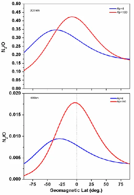
Figure 5. Latitudinal variation of N2/O with magnetic latitude at
Ap=4 and Ap=160 in 300 km and 600 km altitude as obtained from MSIS 90 used in the main frame
The Modelled TEC shows usual diurnal variations. Modelled TEC is maximum on 27th July (~60 units) and 25th July (~50 units) where Ap indices are 154 and 186 respectively. It has been observed that model shows good day-to-day variation of TEC over Trivandrum. Unfortunately, measured TEC data is not available for this period. Diurnal and day-to-day variations of TEC derived from model and TEC measured by GPS is shown in Figure 4a (bottom) during 7-11th November 2004 storm. A usual diurnal variation has been observed with diurnal minimum during pre-sunrise and diurnal maximum in daytime. Modelled maximum TEC is 60 units and measured maximum TEC is 61 units on the day 9th November 2004. Modelled TEC has good agreement of day-to-day variation with observed TEC except on 10th November 2004. The observed TEC on the day 10th November 2004 shows a depression at mid day which isn’t reproduced by the model. The modelled TEC and GPS measured TEC shows good agreement (Figure 4b, bottom) and the correlation coefficient is very high 0.92.
DISCUSSION
During geomagnetic storm/sub storm, solar wind energetic particle directly precipitate into the polar region through the polar cusp giving rise to auroral emissions. Auroral electrojet current subsequently increases resulting in the generation of atmospheric gravity waves (AGW) owing to the joule heating (terrestrial ionosphere is a resistive medium) by the auroral electrojet current system can cause ionospheric perturbations [e.g., Lee et al., 2004; Ding et al., 2008; Lei et al., 2008]. These AGWs propagate towards equator and redistribute the additional energy and momentum globally.
Heating at high latitudes causes the rapid expansion of the neutral atmosphere which causes upwelling, i.e., the motion of air through constant pressure surfaces, resulting in departures from diffusive equilibrium and increases in the mean molecular mass (increases in the ratio of molecular nitrogen N2 to atomic
oxygen O concentration). Figure 5 illustrates the latitudinal variation of N2/O with magnetic latitude at Ap=4 and Ap=160
in 300 km and 600 km altitude as obtained from MSIS 90 which is used in the main model code. It has been observed that increases of N2/O towards equator is more prominent in
Ap=160 than Ap=4. The ratio N2/O is more in 300km altitude.
Mansilla (2006) also reported that changes of neutral composition are responsible of the decreases of electron density observed during the end of long-lasting main phase and recovery phase of the storms. The expansion also results in pressure gradients which modify the global thermospheric circulation. Enhanced equatorward winds transport the composition changes to lower latitudes, so that one sees a ‘‘composition disturbance zone’’ of increased mean molecular mass from high to low latitudes. The equatorward winds are usually stronger at night because the storm-induced winds add the back-ground circulation. They often take the form of equatorward surges or travelling atmospheric disturbances (TADs). (Mayr et al, 1978; Prölss, 1980, 1995; Buonsanto, 1999; Danilov, 2001). During intense geomagnetic storms as considered in this analysis they possibly carry such composition changes to low latitudes.
Basu et al. (2001) analyzed the effects of the great magnetic storm of July 15, 2000 on the equatorial ionosphere by ground based and satellite in situ measurements. They observed a large westward plasma drift in the evening equatorial ionosphere as a result of the ionospheric disturbance dynamo. The IMF Bz turned southward and presumably caused penetration of electric fields to low latitudes. The responses of Equatorial Ionization Anomaly (EIA) to the superstorms of October-November 2003 were investigated using the total electron content (TEC) measured with global positioning system (GPS) receivers in China, Southeast Asia, Australian (CSAA), and the American regions (Zhao, B., et al., 2005).
Enhanced EIA was seen to be correlated with the southward turning of the interplanetary magnetic field Bz. In both the
CSAA and American regions, EIA was intensified, corresponding to a large increase in the F-layer peak height (hmF2) measured by ionosonde and digisonde at middle and equatorial latitudes. However, the enhanced EIA was shown to be more significant during the daytime in the American region, which was associated with a series of large substorms when Bz
deviation in the formation of the crest of anomaly and is confined to 18 to 21 º N. And on the storm days of 8, 9, 10 and 11 November 2004, which are highly disturbed days, the formation of the EIA is disturbed showing the formation of more than one anomaly crest, clearly indicating the effects associated with the disturbed conditions during the storm periods. Similar growth and decay of the EIA has been simulated by the present model (figure 3). Thus, it may be inferred that the storm-induced changes (both increases and decreases) in TEC are significant in the equatorial and low latitude sectors and depend on the strength and phase of the storm and the direction of the IMF Bz. Guozhu et al. (2010) reported the ionospheric observations from a set of in situ satellites and ground based GPS total electron content and scintillation receivers, a VHF radar, and two chains of ionosondes (~300°E and ~120°E, respectively) that provide the evolutionary characteristics of equatorial and low-latitude ionospheric irregularities versus longitude during the storm periods 22–28th July 2004. It is found that the irregularities occurred over a wide longitudinal range, extending from around 300°E to 120°E on storm days 25th and 27th July 2004. On 25th July plasma bubbles (PBs) formed in the premidnight hours in America and postmidnight hours in Southeast Asia. On 27th July the occurrence of irregularities followed the sunset terminator and was observed sequentially after sunset from American to Southeast Asian longitudes. The results indicate that geomagnetic storms triggered the wide longitudinal development of PBs.
The meridional wind circulation also changes both in magnitude and direction following a storm. In general, the equatorial daytime thermosphere is hotter than polar thermosphere during quiet period. Therefore, the meridional wind flows from the equator to polar region during daytime. The reverse happens during nighttime. These quiet time patterns change drastically following geomagnetic storms when the disturbed meridional winds flow from the poles to the equatorial region. In addition to the above effects, current system changes globally and this reflects in the current systems over low- equatorial latitudes also. The solar wind electric field also, on occasions, directly modulates (prompt penetration effect) the equatorial ionospheric electric fields. The changed circulation pattern following a storm results in disturbance dynamo mechanism, which also modulates the equatorial electric fields.
Acknowledgments
The GPS TEC data used in this analysis was obtained as part of the GAGAN project of the Indian Space Research Organisation and the Airport Authority of India.
REFERENCES
Abdu, M. A., Batista, I. S., Walker, G. O., Sobral, J. H. A., Trivedi, N. B., and de Paula, E. R. 1995. Equatorial electric fields during magnetospheric disturbances: Local time/longitude dependencies from recent EITS campaigns, J. Atmos. Terr. Phys., 57, 1065–1072.
Bagiya, M. S., R. Hazarika, F. I. Laskar, S. Sunda, S. Gurubaran, D. Chakrabarty, P. K. Bhuyan, R. Sridharan, B. Veenadhari, and D. Pallamraju 2014. Effects of prolonged southward interplanetary magnetic field on low-latitude
ionospheric electron density, J. Geophys. Res. Space Physics, 119, 5764–5776,doi:10.1002/2014JA020156, 2015.
Basu, S., S. Basu, K. M. Groves, H. C. Yeh, S. Y. Su, F. J. Rich, P. J. Sultan, and M. J. Keskinen, 2001a. Response of the equatorial ionosphere in the South Atlantic region to the Great Magnetic Storm of July 15, Geophys. Res. Lett., 28(18), 3577–3580, doi:10.1029/2001GL013259.
Bhuyan, P K., A. Borgohain, and K. Bhuyan K, Theoretical simulation of electron density and temperature distribution at Indian equatorial and low latitude ionosphere, Advances in Space Research, doi:10.1016/j.asr.2007.05.067, 2007 Blanc, M. and Richmond, A.D. 1980. The ionospheric
disturbance dynamo, Journal of Geophysical Research, 85, 1669–1686.
Buonsanto, M.J. 1999. Ionospheric storms—a review. Space Science Reviews 88, 563–601.
Danilov, A.D. 2001. F2-region response to geomagnetic disturbances. Journal of Atmospheric and Terrestrial Physics, 63, 441–449.
Ding, F., W. Wan, L. Liu, E. L. Afraimovich, S. V. Voeykov, and N. P. Perevalova, 2008. A statistical study of large scale traveling ionospheric disturbances observed by GPS TEC during major magnetic storms over the years 2003– 2005, J. Geophys. Res., 113, A00A01, doi:10.1029/ 2008JA013037.
Fejer, B. G. 1986. Equatorial ionospheric electric fields associated with magnetospheric disturbances in solar wind magnetosphere ~lI:pl. ing, Eds. Y. Kamide and J. A. Slavin, Terra SCientific Pubhshmg Company, Tokyo, pp.519·545. Fejer, B. G., and L. Scherliess, 1997. Empirical models of
storm time equatorial zonal electric fields, J. Geophys. Res., 102(A11), 24,047–24,056, doi:10.1029/97JA02164. Foster, J. C., and F. J. Rich, 1998. Prompt midlatitude electric
field effects during severe geomagnetic storms, J. Geophys. Res., 103, 26367.
Fuller-Rowell, T. M., G. H. Miillward, A. D. 2002. Richmond, and M. V. Codrescu, Storm-time changes in the upper atmosphere at low latitudes, J. Atmos. Sol. Terr. Phys., 64, 1383–1391.
Guozhu Li, Baiqi Ning, Lianhuan Hu, Libo Liu, Xinan Yue, Weixing Wan, Biqiang Zhao, K. Igarashi, Minoru Kubota, Yuichi Otsuka, J. S. Xu and J. Y. Liu, 2010. Longitudinal development of low latitude ionospheric irregularities during the geomagnetic storms of July 2004, Journal of Geophysical Research, Vol. 115, A04304, doi:10.1029/2009JA014830.
Kalita, B. R., R. Hazarika, G. Kakoti, P.K. Bhuyan, D. Chakrabarty, G.K. Seemala, K. Wang, S. Sharma, T. Yokoyama, P. Supnithi, T. Komolmis, C.Y. Yatini, M. Huy, and P. Roy 2016. Conjugate hemisphere ionospheric response to the St. Patrick's Day storms of 2013 and 2015 in the 100°E longitude sector, J. Geophys. Res. Space Physics, 121, doi:10.1002/2016JA023119, 2016.
Lee, C.C., J.Y. Liu, M.Q. Chen, S.Y. Su, H.C. Yeh, and K. Nozaki, 2004. Observation and model comparisons of the traveling atmospheric disturbances over the Western Pacific region during the 6–7 April 2000 magnetic storm, J. Geophys. Res., 109, A09309, doi:10.1029/2003JA010267. Lei, J., A. G. Burns, T. Tsugawa, W. Wang, S. C. Solomon,
2006 geomagnetic storm, J. Geophys. Res., 113, A06310, doi:10.1029/2008JA013090.
Li, G., B. Ning, B. Zhao, L. Liu, W. Wan, F. Ding, J. S. Xu, J. Y. Liu, and Yumoto K. 2009. Characterizing the 10 November 2004 storm time middle latitude plasma bubble event in Southeast Asia using multi instrument observations, J. Geophys. Res., 114, A07304, doi:10.1029/2009JA014057.
Lin, C. H., A. D. Richmond, J. Y. Liu, G. J. Bailey, and B. W. Reinisch, 2009. Theoretical study of new plasma structures in the low latitude ionosphere during a major magnetic storm, J. Geophys. Res., 114, A05303, doi:10.1029/2008JA013951.
Mansilla, G.A., Equatorial and low latitude ionosphere during intense geomagnetic storms, Journal of Atmospheric and Solar-Terrestrial Physics, 68, 2091–2100, 2006.
Martinis, C. R., M. J. Mendillo, and J. Aarons, 2005. Toward a synthesis of equatorial spread F onset and suppression during geomagnetic storms, J. Geophys. Res., 110, A07306, doi:10.1029/2003JA010362.
Mayr, H.G., Harris, I., Spencer, N.W. 1978. Some properties of upper atmosphere dynamics, Reviews of Geophysics and Space Science 16, 539–565.
Misra, P., Enge, P. 2001. Global Positioning System-Signal Measurements and Performance. Ganga-Jamuna Press, Lincoln, Mass.
Moffet, R. J., Bailey, G. J., Quegan, S., Rippeth Y., Samson, A. M. and Sellek, R. 1989. Modelling the ionospheric and plasmaspheric plasma, Phil. Trans. R. Soc.London., 328, 255.
Prölss, G.W. 1980. Magnetic storm associated perturbation of the upper atmosphere: recent results obtained by satellite borne analyzers, Reviews of Geophysics and Space Physics, 18, 183–202.
Raitt, W. J., Schunk, R. W., Banks, P. M. 1975. A comparison of the temperature and density structure in high and low speed thermal proton flow, Planet. Space Sci, 23, 110.
Rama Rao P. V. S., S. Gopi Krishna, J. Vara Prasad, S. N. V. S. Prasad, D. S. V. V. D. Prasad, and K. Niranjan., Geomagnetic storm effects on GPS based navigation, Ann. Geophys., 27, 2101–2110, 2009.
Sahai, Y., et al., Effects of the major geomagnetic storms of October 2003 on the equatorial and low latitude F region in two longitudinal sectors, J. Geophys. Res., 110, A12S91, doi:10.1029/2004JA010999, 2005.
Sastri, J. H., K. B. Ramesh, and H. N. Rangnath Rao, 1992. Transient composite electric field disturbances near dip equator associated with auroral sub storms, Geophys. Res. Lett., 19, 1451–1454.
Sreeja, V., C. V. Devasia, S. Ravindran, T. K. Pant, and R. Sridharan, 2009. Response of the equatorial and low latitude ionosphere in the Indian sector to the geomagnetic storms of January 2005, J. Geophys. Res., 114, A06314, doi:10.1029/2009JA014179.
Stubbe, P.1970. Simultaneous solution of the time-dependent coupled continuity equations, heat conduction equations and equations of motion for a system consisting of a neutral gas, an electron gas and a four component ion gas, J. Atmos. Terr. Phys., 32, 865– 903.
Subrahmanyam P., A. R. Jain, L. Singh, S. C. Garg, 2005. Role of neutral wind and storm time electric fields inferred from the storm time ionization distribution at low latitudes: in-situ measurements by Indian satellite SROSS-C2. Annales Geophysicae, European Geosciences Union, 23 (10), pp.3289-3299.
Torr, D.G. and M.R. Torr, 1979. Chemistry of the thermosphere and ionosphere, J. Atmos. Terr. Phys., 41, 797.
Wang, H., Luhr, H., Ma, S. Y., Weygand, J., Skoug, R. M., and Yin, F. 2006. Field-aligned currents observed by CHAMP during the intense 2003 geomagnetic storm events, Ann. Geophys., 24, 311–324.
Zhao, B., W. Wan, and L. Liu, 2005. Responses of equatorial anomaly to the October–November 2003 super storms, Ann. Geophys., 23, 693–706.