ISSN (e): 2250-3021, ISSN (p): 2278-8719
Vol. 08, Issue 7 (July. 2018), ||V (III) || PP 08-16
Comparative Analysis between Routing Protocol Aodv & Taodv
Rajeev Sharma
1, Dr. Anil Chaudhary
21Dept. Computer Science, Vivekananda global university, Jaipur, India
2Dept. Information Technology, Swami Keshvanand Institute of Technology, Jaipur, India
Corresponding Author: Rajeev Sharma
Abstract:
VANETs (Vehicular Ad-hoc Networks) is a particular kind of (MANET) Mobile Ad-hoc network, in which vehicles on the road from the nodes of the networks. VANETs several applications are used in Intelligent Transportation System. Various kinds of challenges in vehicular communications have been addressed and to recognize. This research paper based on with recital evaluation (AODV) Ad-Hoc on-Demand Distance Vector routing protocols using mobility model Intelligent Driver Model with Intersection Management based on metrics such as packet distribution ratio average end to end delay and throughput. In this research paper we also present how the sumo simulator communicates with Network Simulator. The result of sumo as a text file.Ns2 and Sumo are open access tools. Research methodology based on NS-2 and sumo simulator open access simulator. The major aim of this paper is to improve the enhancement and performance of AODV protocol. In this investigation, the performance of AODV has been analyzed by means of packet delivery ratio, E2E delay, packet damage ratio.Keywords:
VANET, AODV, SUMO, NS-2.--- --- Date of Submission: 28-06-2018 Date of acceptance: 13-07-2018 ---
---I.
INTRODUCTION
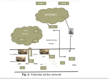
VANETs are conjunction of movable nodes, vehicles operational with on OBU and static nodes called road side unit (RSU) attach to in infrastructure. On board unit and Road side unit have wired/wireless communication capabilities. Fundamentally Vanet is two kinds of transmission environments Vehicle to Road and Vehicle to Vehicle.
Vanets transmission allows various types of applications. These are mainly classified as safety applications, comfort applications and Administrator applications i.e. [3].A particular choice of route is fixed using routing algorithms. In this research paper describes proactive AODV routing protocol algorithm.
The research paper is structured as follows. Segment II Routing protocols categories. Segment III Research Methodology used segment IV shows results and analysis. Finally conclusion & future scope in the paper Section V.
II.
ROUTING PROTOCOLS VANETS
A routing protocol regularize the way of exchanging information in two communication existence; it includes the process in establishing a route, decision in forwarding, and recovering or action in maintaining the route from routing failure. Routing protocol are two types topology-based and geographic (position-based). Topology routing protocols use associations information to forward the packet where as geographic routing uses the information about the location of position to forward the packet. Topology based routing divided again be proactive or reactive i.e. [8]. Proactive protocol uses the routing table for dissemination of message whereas reactive protocol construction the route only when it is required.
AODV Routing protocol is a unicast reactive routing protocol for ad-hoc network. AODV is maintained the active path information only in routing tables at all the nodes. The next hop routing table at all nodes hold information of destinations to which the route is submitted currently. Whenever the route is not been used or not reactivated for a pre-specified expiration time then routing table entry expires.
III. RESEARCH METHODOLOGY USED
For this investigation, we are used two simulator sumo simulator and Ns-2. Sumo simulator and network simulator are an open source platform specific for VANETs which is useful to generate simulation results. A Motility trace is generated as output with sumo simulator; this motility trace is used by a simulation simulator such as ns-2 to simulate reasonable vehicle movement.
A. Sumo Simulator
“Simulation of Urban Mobility “ is extremely portable, microscopic road traffic simulation package designed to handle wide road network .It permit to simulate how a given traffic demand which based on single vehicles moves throughput a given road network.
The simulation allows to trace a wide set of traffic management topics. It is exclusive microscopic: every vehicle is modeled explicitly, has own route and moves separately throughput the network.
B. Network Simulator
For Network Simulator we use NS-2 an open source simulator i.e. [6].It is distinct event simulator. A sufficient support is provided by NS-2 for routing, simulation of TCP/UDP and multicast protocols. Network simulator Ns-2 provides support for both wireless and wired networks. Table.1simulation area specifications are presented for NS2 i.e. [2].
TABLE 1: NS2 SIMULATION SETTINGS
IV. RESULT AND ANALYSIS
We have selected routing protocol is AODV .These routing protocols we calculated metrics such as Throughput, and Average end to end Delay and Packet Delivery Ratio.
Operating System Ubuntu 14.04 Simulator Network2.35,SUMO Simulation time 100 s
STATUS 1: Throughput of sending packets AODV & TAODV
Fig. 2: Throughput of sending packets AODV
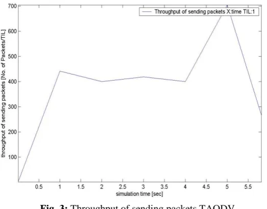
In this graph demonstrate throughput abruptly rises to 450 packets TIL in exclusively 01 sec and then it persists to give throughput of 450 packets TIL approx. For approximately 04 sec, then it instantly goes abruptly rise to 700 packets TIL and remain there with appreciable variation for about 2secs approx. Then it instantly rise down at 06 sec., it afterwards drops to 500 packets/TIL .This can be contained as “the amount of packets sent per unit time reduces .The packets sent are average in the beginning because in the opening stage of VANET, the nodes are sending beacons in order to setup the network ”.
Fig. 3: Throughput of sending packets TAODV
STATUS 2: Throughput of receiving packets AODV & TAODV
Fig.4: Throughput of receiving packets AODV
In this graph demonstrate throughputs abruptly rise to 350 packets TIL in exclusively in 01 sec and then it persists to give throughput of little more to 350 packets TIL approx. For approximately 04 sec, then it instantly goes abruptly rise to 1050 packets TIL with appreciable variation for about 1secs approx. Then it instantly rise down at 06 sec., it afterwards drops to 950 packets/TIL .This can be contained as “the amount of packets received per unit time reduces .The packets received are average in the beginning because in the opening stageof VANET, the nodes are receiving beacons in order to setup the network ”.
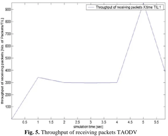
Fig. 5. Throughput of receiving packets TAODV
In this graph demonstrate throughputs abruptly rise to 350 packets TIL in exclusively in 01 sec and then it persists to give throughput of little more to 350 packets TIL approx. For approximately 04 sec, then it instantly goes abruptly rise to 950 packets TIL with appreciable variation for about 1 sec approx. Then it instantly rise down at 06 sec., it afterwards drops to 450 packets/TIL .This can be contained as “the amount of packets received per unit time reduces .The packets received are average in the beginning because in the opening stage of VANET, the nodes are receiving beacons in order to setup the network ”.
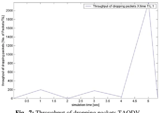
STATUS 2: Throughput of dropping packets AODV & TAODV
To study the difference between throughput of AODV and TAODV, we compare the resultant throughput from both of the protocols one by one. The final result is shown by the separate graph for both of the cases. The graph demonstrates the simulation time which is aligned with the throughput of dropping packets. Throughput of dropping packets is the amounts of packets dropped for every unit TIL. Simulation instant is deliberate in seconds.
Fig. 6: Throughput of dropping packets AODV
In this graph demonstrate throughputs solely rise to 50-100 packets TIL in exclusively in 01 sec and then it dropped to zero in the next second. Then in the simulation time of 30 sec, it raises same as earlier to over 50-100 packets/TIL and reduces to zero for 4 times For approximately 04 sec, then it instantly goes abruptly rise to 2100 packets TIL with appreciable variation for about 1 sec approx. Then it instantly rise down at 06 sec., it afterwards drops to 20500 packets/TIL .This can be contained as “the amount of packets dropped per unit time reduces .The packets dropped are lower in the beginning because in the opening stage of VANET, the nodes are dropped beacons in order to setup the network”.
Fig. 7: Throughput of dropping packets TAODV
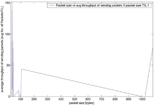
STATUS 4: Packet Size V/s Average Throughput of sending packets AOVDV & TAOD
To study the difference between average throughput of sending packets for AODV and TAODV in reference of packet size, we compare the resultant throughput from both of the protocols one by one. The final result is shown by the separate graph for both of the cases. The graph demonstrates the simulation time which is aligned with the average throughput versus packet size. An average throughput packet is the amounts of in general ration of packets received for every unit TIL. Simulation instant is deliberate in seconds.
Fig. 8: Packet Size versus Average throughput of sending packets AODV
In this graph demonstrate a relation between average throughputs of sending packets (average number of packets /TIL) and Packets size in the bytes. This graph shows that average throughput of small sized packets (1-20 bytes) is more (20 packets/TIL) than huge sized packets1000 bytes).The initial value of the graph starts from zero and it reach to 10 average packets /TIL where the value for this on x axis is 100 bytes which is packer size. It is observed that the highest value on the y axis immediately rise to approx. 40 packets (average number of packets /TIL) and packet size is 100 bytes at the moment shown by y axis. At the next values declined as per the increasing packet size. At the last on the size of 1000 bytes packet size the average throughputs was zero. So we can say that as per the graph for sending packets average throughput of small sized packets (1-20 bytes) is more (20 packets/TIL) than huge sized packets1000 bytes)”.
Fig. 9: Packet Size V/s Average throughput of sending packets for TAODV
bytes at the moment shown by y axis. At the next values declined as per the increasing packet size. At the last on the size of 1000 bytes of packet size the average throughputs was zero. So we can say that as per the graph for sending packets average throughput of small sized packets (1-25 bytes) is more (25 packets/TIL) than huge sized packets1000 bytes) .
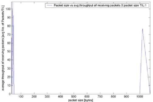
STATUS 5: Packet Size V/s Average Throughput of receiving packets AODV & TAODV
This section of the study gives the difference between average throughput of receiving packets for AODV and TAODV in reference of packet size, we compare the resultant throughput from both of the protocols one by one. The final result is shown by the separate graph for both of the cases. The graph demonstrates the simulation time which is aligned with the average throughput versus packet size. An average throughput packet is the amounts of in general ration of packets received for every unit TIL. Simulation instant is deliberate in seconds.
Fig. 10: Packet Size V/s Average throughput of receiving packets AODV
In this graph demonstrate a relation between average throughputs of receiving packets (average number of packets /TIL) and Packets size in the bytes. This graph shows that average throughput is maximum for diminutive sized packets and zero for packet size of range 90-1000 bytes. The initial value of the graph for average throughput of receiving packets starts from zero and it is continue for large time. It is observed that the highest value on the y axis immediately rise to approx. 60 packets (average number of packets /TIL) and packet size is 100 bytes at the moment shown by y axis. At the next values declined as per the increasing packet size. At the last on the size of 1000 bytes of packet size the average throughputs was zero. So we can say that as per the graph for receiving packets the average throughput is maximum for diminutive sized packets and zero for packet size of range 90-1000 bytes.
In this graph demonstrate a relation between average throughputs of receiving packets (average number of packets /TIL) and Packets size in the bytes. This graph shows that average throughput is maximum for diminutive sized packets and zero for packet size of range 90-1000 bytes. The initial value of the graph for average throughput of receiving packets starts from zero and it is continue for large time. It is observed that the highest value on the y axis immediately rise to approx. 75 packets (average number of packets /TIL) and packet size is 100 bytes at the moment shown by y axis. At the next values declined as per the increasing packet size. At the last on the size of 1000 bytes of packet size the average throughputs was zero. So we can say that as per the graph for receiving packets the average throughput is high for diminutive sized packets and zero for packet size of range 90-1000 bytes.
There is comparison of general environmental statistics of routing protocol AODV with the clone of the AODV, which is named as TAODV. Parameters on which these comparisons get performed are Average throughput. Packet sent, Packet Received, Packet dropped and packet fractions. The statistics for both the protocols are given below:
Table 2: Throughput and Packet Delivery with AODV & TAODV
Experimental Information (Screen Shots)
The screen shots for the experimental and observations for the routing protocol AODV and cloned routing protocol TAODV are as follows:
Fig. 12: Screen Shots-1 for Experimental
V.
CONCLUSION & FUTURE SCOPE
experimental according to routing protocol. The parameters taken for the study were packet drops, delay time, packet size, throughput etc.
REFERENCES
[1]. M. Guezouri and A. Bennaoui, Performance Evaluation of Routing Protocols in Vehicular Networks. I. J. Computer Network and Information Security, 2013, 10, 11-16.
[2]. K. Venkateswarlu, G. Murali, Performance Evaluation Of Dsdv, Aodv Routing Protocols In Vanet,IJRET: International Journal of Research in Engineering and Technology eISSN: 2319-1163 | pISSN: 2321-7308, May 2015.
[3]. Tajinder Kaur, A. K. Verma, Simulation and Analysis of AODV routing protocol in VANETs,International Journal of Soft Computing and Engineering (IJSCE) ISSN: 2231-2307, Volume-2, Issue-3, July 2012.
[4]. Anuj K., Gupta Harsh Sadawarti and Anil K. Verma “Performance analysis of AODV, DSR & TORA Routing Protocols ,IACSIT International Journal of Engineering and Technology, Vol.2, No.2, April 2010 ISSN: 1793-8236.
[5]. http://vanet.eurecom.fr.
[6]. NS-2- http://www.isi.edu/nsnam/ns.
[7]. IDM-IM (Intelligent Driver Model with Intersection Management) VanetMobisim manual.
[8]. Lee, K. C., Lee, U., & Gerla, M. (2010), “Survey of RoutingProtocols in Vehicular Ad Hoc”. Networks”,Advances in Vehicular Ad-Hoc Networks:Developments and Challenge, Watfa, M. (Ed.), (pp. 149-170), 2010.
[9]. Meenakshi Diwakar1and Sushil Kumar2,” an energy efficient level based clustering routing protocol for wireless sensor networks”, IJASSN, Vol 2, No.2, Apriln 2012.
[10]. http://www.nsnam.com [11]. https://www.nsnam.org [12]. http://www.dlr.de [13]. http://sumo.dlr.de/wiki
[14]. Anas Abu Taleb ,“VANET Routing Protocols and Architectures: An Overview” Journal of Computer Science 2018, 14 (3): 423.434, DOI: 10.3844/jcssp.2018.423.434.
[15]. Md. Mamunur Rashid , Prithwiraj Datta “Performance Analysis of Vehicular Ad Hoc Network (VANET) Considering Different Scenarios of a City”, International Journal of Computer Applications (0975 – 8887) Volume 162 – No 10, March 2017.
[16]. Ramesh C. Poonia, DeepshikhaBhargava,” A Review of Coupling Simulator for Vehicular Ad-hoc Networks” I.J. Information Technology and Computer Science, 2016, 5, 44-51.