RSS-based Near-Collinear Anchor aided Positioning Algorithm for Ill-conditioned Scenario

International Journal of Wireless Communications and Mobile Computing 2014; 2(1): 18-22

Published online February 20, 2014 (http://www.sciencepublishinggroup.com/j/wcmc) doi: 10.11648/j.wcmc.20140201.13

RSS-based near-collinear anchor aided positioning

algorithm for Ill-conditioned scenario

Senka Hadzic

1, 2

, Du Yang

1

, Manuel Violas

1, 2

, Jonathan Rodriguez

1

1

Instituto de Telecomunicações, Aveiro, Portugal 2

Universityof Aveiro, Aveiro, Portugal

Email address:

[email protected] (S. Hadzic), [email protected] (D. Yang), [email protected] (M. Violas), [email protected] (J. Rodriguez)

To cite this article:

Senka Hadzic, Du Yang, Manuel Violas, Jonathan Rodriguez. RSS-based Near-Collinear Anchor aided Positioning Algorithm for Ill-conditioned Scenario. International Journal of Wireless Communications and Mobile Computing. Vol. 2, No. 1, 2014, pp. 18-22. doi: 10.11648/j.wcmc.20140201.13

Abstract:

The conventional Received Signal Strength (RSS) based positioning algorithms such as Least Square (LS) and Weighted LS (WLS) produce significant estimation errors when the anchor nodes positions approach a collinear scenario. In this paper, we propose the CAP (Collinear Anchor aided Positioning) algorithm to provide robust positioning performance under ill-conditioned matrix conditions, whilst contributing toward overall low computational complexity. The CAP algorithm outperforms traditional approaches such as the maximum likelihood algorithm, LS and WLS among others.

Keywords:

Ill-Conditioned, Collinear Anchors, Unbiased Estimate, CRLB

1. Introduction

Wireless position estimation (locating a node using measurements from surrounding location-known anchors) is increasingly becoming a prominent feature for intelligent services and applications. There are mainly three popular estimation approaches: lateration, angulation, and mapping. Lateration techniques compute the position of an object by measuring its distances from multiple anchors. The distances could be obtained from received signal parameters such as Time of Arrival (ToA) [1]-[2] or Received Signal Strength (RSS) [3]. The target node position can be computed using estimation algorithms such as Least Square (LS) [4], Weighted Least Square (WLS) [5], Maximum Likelihood (ML) [3], etc. Another popular technique is angulation, which uses the measured Angle of Arrival (AoA) [6] to determine the target node position. The third one is mapping, which matches the measured signal parameter (e.g RSS) with a database consisting of the same type of signal parameters at known positions [7] so as to determine the position. The RSS-based lateration technique is the most practical in terms of implementation since it does not require any synchronization, antenna arrays or external database. In this paper, without loss of generality we will focus on RSS-based lateration technique in a 2-dimensional space. The geometric method can be applied to ToA based distance estimates, without any restrictions.

One limitation of lateration technique is that it requires distance measurements from at least 3 non-collinear anchors for calculating an object’s position in 2-dimensional space. The accuracy of above-mentioned LS and WLS significantly degrades when the anchors are approaching collinear. The main reason for this degradation is that these two positioning algorithms involve matrix inversions which results in significant error injection when the matrix is ill-conditioned. The accuracy of high-complexity ML algorithm also degrades as well.

The remainder of the paper is organized as follows: we present the related work in Section 2and our motivation to investigate the problem of collinear anchors; in Section 3 we describe the target scenario, RSS distance estimation, and some conventional positioning algorithms; Section 4 explains our proposed algorithm, namely the collinear anchors aided positioning algorithm; Section 5 evaluates the performance through simulations and finally, Section 6 concludes the paper.

2. Related Work

The problem of anchor placement is a well-known subject in localization literature [12-14]. Whether the localization algorithm is statistical and uses the Cramer-Rao lower bound as performance metric [13-14], or it introduces a new confidence metric for geometrical localization such as trilateration [12], the conclusions are similar - the best performance is given when anchor nodes are well separated around the target. One of the anchor constellations that have the biggest negative impact on localization performance is the collinear case, and several works have adopted methods to identify and discard such setups. It has been referred to as the ‘pathological’ case [8], and the goal is to avoid it. Specific lower bounds on thedegree of collinearity of anchor nodes sufficient to achieve optimal localization results have been proposed in [15]. The metric to measure collinearity is the height of the anchor triangle. The impact of anchor placement has also been studied in [16].

To our knowledge, there has not been work done in actually exploiting the near collinear case for localization purposes.

3. Preliminaries

3.1. Target Scenario

The target scenario we consider in this paper is illustrated in Fig. 1 that depicts the target node position in a

2-dimensional space with Nnear collinear anchors.

Figure 1.Target scenario.

The target node

T

is located in a 2-dimensional space with

unknown coefficients (x,y). There are N fixed near collinear

located anchors. In order to quantify the degree of collinear

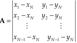
between anchor nodes, we introduce the matrix A_{as in [8],}

which is formulated as:

1 1

2 2

1 1

− −

−

−

−

−

=

−

−

A

⋮

⋮

N N

N N

N N N N

x

x

y

y

x

x

y

y

x

x

y

y

(1)

This matrix contains information about geometrical configuration of anchor nodes. We use the condition number

of matrix cond(A) as an indicator of colinearity: in the

extreme case when all three anchors are collinear, the matrix is singular and the condition number is infinite. If the condition number is too large, the matrix (in our case the scenario) is said to be ill-conditioned.

3.2. RSS-Based Distance Estimation

There are several methods for distance estimation, such as RSS [4], ToA [2], etc. Even though in practice it has been shown that the RSS ranging performs well in addition to location maps (fingerprinting), we adopt RSS method in this paper due to its simplicity. It is still most easy-to-apply method for practical systems, because there is no need for any additional hardware, neither for synchronization.

Supposed that the anchors Ri transmit a signal, and the

long-term averaged received signal strength at reference

distance d0 is P0 (dBm), the long-term averaged received

signal strength Pi at the target node T is formulated as

α σ

= − +N 2

0

0

( ) ( ) 10 log i (0, )

i i

d

P dBm P dBm

d (2)

Here direpresents the distance between Ri and T,

α

represents the path-loss constant, and N(0, ) represents

log-normal shadow fading variance. Employing the unbiased estimator proposed in [9]-[10], and based on the

results of [11], the unbiased estimate of di2is:

λ α α

− −

=

ɶ

2

2

2 2

2

i i

r

i

d

e

(3)

In the above equation, the element

2 2 2

0 0

0.1ln(10)( ) αln( ) λ 0.01(ln(10)) σ .

= − − =

i i i i

r P P d ,

Moreover, the variance of the estimation is formulated as:

λ α

=

−

ɶ

2 2

4

2 4

var(

)

(

1)

i

i i

d

d e

(4)

Equation (4) demonstrates that the variance grows

exponentially with the shadowing parameter [11]. Since

20 Senka Hadzic et al.: RSS-based Near-Collinear Anchor aided Positioning Algorithm for Ill-conditioned Scenario

3.3.Conventional Positioning Algorithms

Having the estimated distances dɶ_i2 and the knowledge of

anchors’ locations, the target node is capable of estimating

its own location coefficients (x, y) by exploiting the

relationship (xi -x)2+(yi- y)2 = ɶ2

i

d . The most common

estimation algorithm is (linear-) Least Square (LS) [6], and its improved versions including the Weighted Least Square (WLS) [7], iterative least square (ILS) [9] etc. However, the

above-mentioned algorithms require at least 3

well-conditioned anchors. The Maximum-likelihood (ML) estimation algorithm [4] does not have this constraint, but it requires iterative operations, which results in high computational complexity. Motivated by the insufficiency of current estimation algorithms, we propose a new Collinear Anchor aided Positioning (CAP) estimation algorithm, which is described in the next section.

4. Collinear Anchor Aided Positioning

Algorithm

In this section, we describe the proposed algorithm given

a scenario with N = 3 anchor nodes. The proposed algorithm

can be extended to N> 3scenario by first selecting 3 anchors

having the most reliable estimation of distance, meaning having the smallest estimation variance according to Equation (4).

Supposed there are three near collinear anchors R1,R2 and

R3, ≤ ≤

ɶ2 ɶ2 ɶ2

1 2 3

var(d ) var(d ) var(d ), the proposed CAP algorithm is detailed as follows:

Step 1: Employ the typical LS algorithm; obtain an initial estimation of the target node’s location, which is represented as₍ɶ(1)_,ɶ(1)₎

x y .

Step 2: By choosing two first two anchorsR i_i, =

{ }

1, 2 ,

we have the following two equations:

− + − =

− + − =

ɶ

ɶ ɶ

ɶ

ɶ ɶ

2 2 2

1 1 1

2 2 2

2 2 2

( ) ( )

( ) ( )

x x y y d

x x y y d (5)

whereɶ2

i

d is the estimated distance between node Ri and

node T using the unbiased algorithm of Equation (3).

Coordinates _{( , )x y}ɶ ɶ _{represent the estimated coordinates.}

Since the anchors lie on the line l, without loss of generality,

we choose the x-axis in parallel with this line lto simplify the

notations as shown in Fig.1. This condition can be easily achieved using transformations as translation, rotation and

reflection. Hence, we havey1 = y2. By subtracting those two

equations, after simple rearrangement we get an estimation of x:

− − −

=

−

ɶ ɶ

ɶ

2 2 2 2

(2 ) 2 1 2 1

1 2

( )

2( )

d d x x

x

x x (6)

By substituting

x

ɶ

( 2 )into Equation (5), we have:

if 0

if < 0 if 0

if < 0

+

−

 _{− − ≥}

 _{+ − −}

=

− −



 _{− − ≥}

 _{− − −}

=

− −



ɶ

ɶ _ɶ ɶ

ɶ

ɶ _ɶ

ɶ

ɶ _ɶ ɶ

ɶ

ɶ _ɶ

(2 )

2 2

(2)

2 2

1 1

(2 ) 1 1 1

( 2)

2 2

1 1 ( 2)

2 2

(2 )

2 2

1 1

(2 ) _{1 1 1}

( 2)

2 2

1 1

( ) ( )

( ) 0

( ) ( )

( ) 0

d x x y d x x

y

d x x

d x x y d x x

y

d x x

(7)

From (7) we conclude that two estimates _yɶ( )± _{can be}

calculated. In cases where the solution is an imaginary number, e.g., when there is no solution, we decided to

assume the valuey = 0. This situation appears in case of a

high

σ

2 value. We obtain two second-step estimations of y:

+

ɶ( 2 )

y and_yɶ( 2 )− _.

Step 3: So far we have three estimation results:_(xɶ(1)_,yɶ( 1)_),

+

ɶ( 2 ) ɶ( 2 )

(x ,y ), and_(xɶ( 2 )_,yɶ( 2 )−_{). The final estimation is chosen} as follows:

=

ɶ

( 3)

ɶ

( 2 )

x

x

(8)

{

}

+ −

+ −

= − −

ɶ ɶ

ɶ ɶ ɶ ɶ ɶ

( 2 ) ( 2 )

(3) ( 2 ) (1) ( 2 ) (1)

,

arg min ,

y y

y y y y y ₍₉₎

The advantage of the CAP algorithm is that it avoids ill-conditioned matrix inversion. Hence it outperforms traditional localization algorithms when having near collinear anchors as shown in the next section.

5. Analysis and Simulation Results

In order to evaluate the performance of our proposed algorithm, we perform simulations in MATLAB. We compare the performance of the CAP algorithm to the state-of-the-art algorithms, specifically LS, WLS and ML, and also include the Cramér-Rao lower bound (CRLB) as a performance indicator. We consider a scenario having the minimum number of anchors (three) and one target. The

target T is placed at fixed coordinates (50, 50), namely in the

center of a 100 x 100 m square area. We assume that the path loss value is the same throughout all area, namely α = 3. We compute the root mean square error (RMSE) for different algorithms by running 1000 simulation runs, for shadowing variance values between -20 and 20 dB.

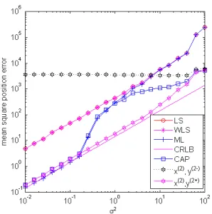
In the first simulation, three anchors are fixed at coordinates (20, 20) and (70, 20), and (90, 30), results in

matrix condition number cond(A)=10.9. The position

estimation RMSE versus shadowing variance using different positioning algorithms is illustrated in Fig.

low shadowing scenario 0.1, the RMSE using LS and

WLS is 6.75 meter, whilst using the proposed CAP the RMSE is 1.37 meter. Note that Fig. 2 has logarithmic scale. The proposed algorithm is about 5 times more accurate than the LS and WLS algorithms. Moreover, at medium

scenario 1, the performance of the proposed CAP

algorithm is reduced, but still showing bett

than the LS and WLS algorithm. Furthermore, at high

shadowing cases 10 , the estimation error using CAP

becomes again significantly better than the conventional LS and WLS. The performance of CAP algorithm is comparable with the performance of the ML algorithm in low and medium shadowing conditions. The ML estimator is usually implemented using the expectation-maximization (EM) iterative algorithm, which may converge to a local maximum depending on starting values. The relatively poor performance of ML in high shadowing scenario shown in Fig. 2 is due to using the EM algorithm, and using LS estimates as its starting value.

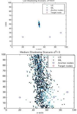
As illustrated in Fig. 2, the mean square error using ML is close to the CRLB when the shadowing variance is low, which means the distance estimation is relatively accurate. It increases as the shadowing variance increases, and finally converge to the curve using LS estimation. To better illustrate this phenomena, we demonstrate the spatial distribution of the estimated results using LS and ML for an ill-conditional scenario in Fig. 3. The three anchor nodes are located at fixed locations, namely (20, 20) and (70, 20), and (90, 30) (all in meters), while the target is in the center of the area, at coordinate (50,50).The lower the shadowin variance, the estimations are less scattered around the mean value.

Figure 3. Three anchors nodes, the target node, the estimates using LS, and the estimates using ML (implemented via EM iterative algorithm), when the shadowing variance is 0.01 (upper) and 6 (bottom)

In the first simulation, three anchors are fixed at coordinates (20, 20) and (70, 20), and (90, 30), results in )=10.9. The position estimation RMSE versus shadowing variance using different Fig. 2. It shows that at , the RMSE using LS and WLS is 6.75 meter, whilst using the proposed CAP the Note that Fig. 2 has logarithmic scale. The proposed algorithm is about 5 times more accurate than the LS and WLS algorithms. Moreover, at medium , the performance of the proposed CAP algorithm is reduced, but still showing better performance than the LS and WLS algorithm. Furthermore, at high , the estimation error using CAP becomes again significantly better than the conventional LS and WLS. The performance of CAP algorithm is comparable nce of the ML algorithm in low and medium shadowing conditions. The ML estimator is usually maximization (EM) iterative algorithm, which may converge to a local maximum depending on starting values. The relatively poor formance of ML in high shadowing scenario shown in 2 is due to using the EM algorithm, and using LS

the mean square error using ML is close to the CRLB when the shadowing variance is low, ich means the distance estimation is relatively accurate. It increases as the shadowing variance increases, and finally converge to the curve using LS estimation. To better illustrate this phenomena, we demonstrate the spatial results using LS and ML for an 3. The three anchor nodes are 20) and (70, 20), and (90, 30) (all in meters), while the target is in the center of the lower the shadowing variance, the estimations are less scattered around the mean

Three anchors nodes, the target node, the estimates using LS, and the estimates using ML (implemented via EM iterative algorithm), when the

e is 0.01 (upper) and 6 (bottom).

The ML estimates are capable of converging to the true target nodes when the shadowing value is

ML estimates become similar to the LS estimates in a scenario with higher shadowing. Although randomly choosing multiple starting values can improve this drawback of EM, it still cannot guarantee the convergence to the global optimum, while it significantly increases the complexity. To sum up, ML should outperform our proposed algorithm in However, using the practical EM algorithm, ML becomes worse than our proposed algorithm in practice. In a high shadowing scenario, the performance of the ML

converges to the LS performance since it employs the LS estimate as its initial value before iteration. Having this implementation in mind, our proposed CAP algorithm slightly outperforms the ML solution at high values of shadowing variance.

On the other hand, the proposed CAP algorithm is much more computationally efficient. Since the ML involves computationally demanding mathematical operations such as matrix inversion and matrix multiplication coupled with the iterative procedure, its complex

3 * ( )

iter

N O N , where N_iter is the number of iterations (in

our simulations we usedN_iter

anchor nodes. On the other hand, the CAP algorithm only involves simplest algebraic operations, such as addition, subtraction and division. Therefore its complexity is in the order ofO N( ).

Figure 4. Condition number as metric for ill and the gain of CAP vs. LS and WLS(bottom)

In the second simulation, the first two anchors remain at (20, 20) and (70, 20), while the third anchor is moved along a circle with radius 45m in steps of 15

show the plot of the condition number versus the angle of the third anchor with respect to line

Furthermore, we compute the

RMSE using LS/ WLS and the RMSE using CAP. Hence, if

gain 1, the proposed CAP algorithm provides less or equal

estimation accuracy. If gain> 1, the proposed CAP algorithm

provides higher estimation accuracy compared to the capable of converging to the true target nodes when the shadowing value is 0.01.However, the ML estimates become similar to the LS estimates in a scenario with higher shadowing. Although randomly choosing multiple starting values can improve this drawback of EM, it still cannot guarantee the convergence to the global t significantly increases the complexity. To sum up, ML should outperform our proposed algorithm in However, using the practical EM algorithm, ML becomes worse than our proposed algorithm in practice. In a high shadowing scenario, the performance of the ML algorithm converges to the LS performance since it employs the LS estimate as its initial value before iteration. Having this implementation in mind, our proposed CAP algorithm slightly outperforms the ML solution at high values of

the other hand, the proposed CAP algorithm is much more computationally efficient. Since the ML involves computationally demanding mathematical operations such as matrix inversion and matrix multiplication coupled with the iterative procedure, its complexity will be in the order of

iter is the number of iterations (in

20

iter

N = ), and N the number of

anchor nodes. On the other hand, the CAP algorithm only simplest algebraic operations, such as addition, subtraction and division. Therefore its complexity is in the

Condition number as metric for ill-conditioned scenario (top), and the gain of CAP vs. LS and WLS(bottom).

In the second simulation, the first two anchors remain at (20, 20) and (70, 20), while the third anchor is moved along

a circle with radius 45m in steps of 15⁰_{. In Fig.4 (top) we}

show the plot of the condition number versus the angle of the

third anchor with respect to line l for a full 360⁰ _circle.

Furthermore, we compute the gain as the ratio between the

22 Senka Hadzic et al.: RSS-based Near-Collinear Anchor aided Positioning Algorithm for Ill-conditioned Scenario

LS/WLS algorithm. As we can see from Fig. 3, by setting

0.1_{, our CAP algorithm outperforms both the LS and}

WLS for ill-conditioned scenarios having large matrix condition value.

The gain over LS is larger than the gain over WLS, which indicates that the WLS is more robust to the ill-conditioned scenario than LS algorithm. We can also conclude that the condition number is a good indicator of accuracy.

6. Conclusion

We have proposed the CAP algorithm that performs well under ill-conditioned scenarios where the anchor nodes are almost collinear; which can be likely in public safety scenarios. The proposed algorithm has been shown to provide up to seven times more accuracy than the traditional LS and three times more than WLS algorithms, whilst showing almost three orders of magnitude less in terms of complexity.

In our future work we intend to apply different channel parameters for each link, since the identical channel model does not represent the realistic indoor channel conditions in the best way. However, our assumption serves well for the evaluation of the proposed method. We also aim at analyzing different simulation setups, for various geometric configurations of anchor nodes and location-unaware nodes.

Acknowledgment

This work has been supported in part by the Portuguese Foundation for Science and Technology (Fundação para aCiência e Tecnologia - FCT) under grant number SFRH / BD / 61023 / 2009.

The research leading to these results has received funding from FEDER through Programa Operacional Factores de Competitividade - COMPETE and from National funds from the Portuguese Foundation for Science and Technology (Fundação para a Ciência e Tecnologia – FCT) under the project PTDC/EEA-TEL/119228/2010 – SMARTVISION.

References

[1] N. A. Alsindi, K. Pahlavan, and B. Alavi, “An Error Propagation Aware Algorithm for Precise Cooperative Indoor Localization”, in Proceedings of IEEE Military Communications Conference MILCOM 2006, pp. 1-7, Washington, DC, USA, October 2006.

[2] X. Wang, Z. Wang and B. O’Dea, “A TOA-based location algorithm reducing the errors due to non-line-of-sight (NLOS) propagation”, in IEEE Transactions on Vehicular Technology, vol.52, issue 1, pp.112-116, Jan. 2003.

[3] N. Patwari, A.O. Hero, M. Perkins, N.S.Correal, R.J. O'Dea, “Relative location estimation in wireless sensor networks,” in IEEE Transactions on Signal Processing, vol. 51, no. 8, pp. 2137-2148, Aug. 2003.

[4] I. Guvenc, S. Gezici, and Z. Sahinoglu, “Fundamental limits and improved algorithms for linear least-squares wireless position estimation,” in Wiley Wireless Communications and Mobile Computing, Sep. 2010.

[5] P. Tarrio, A.M. Bernardos, J.A. Besada and J.R. Casar, “A new positioning technique for RSS-Based localization based on a weighted least squares estimator,” in Proc of IEEE International Symposium on Wireless Communication Systems, Reykjavik, Iceland, pp.633-637, Oct. 2008.

[6] P. Rong and M. L. Sichitiu, “Angle of Arrival Localization for Wireless Sensor Networks ”, in Proceedings of 3rd Annual IEEE Communications Society on Sensor and Ad Hoc Communications and Networks (SECON '06), vol.1, pp.374-382, Sept. 2006.

[7] P. Bahl, and V. N. Padmanabhan, “RADAR: An in-building RF-based user location and tracking system,” in InfoCom 2000, Tel Aviv, Israel, pp.775-784, March 2000.

[8] J. Liu, Y. Zhang and F. Zhao, “Robust Distributed Node Localization with Error Management”, in Proc. of the 7th ACM international symposium on Mobile ad hoc networking and computing (MobiHoc ’06), pp.250-261, New York, USA, 2006.

[9] H.C.So and L.Lin, "Linear least squares approach for accurate received signal strength based source localization," IEEE Transactions on Signal Processing, vol.59, no.8, pp.4035-4040, August 2011.

[10] L.Lin and H.C.So, "Best linear unbiased estimator algorithm for received signal strength based localization," Proc. 2010 European Signal Processing Conference, Barcelona, Spain, pp.1989-1993, Aug. 2011.

[11] S.D. Chitte, S. Dasgupta and Z. Ding, “Distance estimation from received signal strength under log-normal shadowing: bias and variance,” IEEE Signal Processing Letters, vol.16, no.3, pp.216-218, Mar. 2009.

[12] Zheng Yang; Yunhao Liu, "Quality of Trilateration: Confidence-Based Iterative Localization," IEEE Transactions on Parallel and Distributed Systems, vol.21, no.5, pp.631,640, May 2010.

[13] Stefan O. Dulman, AlineBaggio, Paul J.M. Havinga, and Koen G. Langendoen, “ A geometrical perspective on localization,” Proceedings of the first ACM international workshop on Mobile entity localization and tracking in GPS-less environments (MELT '08). ACM, New York, NY, USA, 85-90, 2008.

[14] Salman, N.; Maheshwari, H.K.; Kemp, A.H.; Ghogho, M., "Effects of anchor placement on mean-CRB for localization," Ad Hoc Networking Workshop (Med-Hoc-Net), 2011 The 10th IFIP Annual Mediterranean , vol., no., pp.115,118, 12-15 June 2011.

[15] Kunz, T.; Tatham, B., "Localization in Wireless Sensor Networks and Anchor Placement," J. Sens. Actuator Netw. 1, no. 1, pp. 36-58, 2012.