t-test Using STATA Software

(1)

CORRESPONDING AUTHOR: Prof. Dato Dr. Munn Sann Lye, Department of Community Health, Faculty of Medicine and Health sciences, Universiti Putra Malaysia, Serdang, 43400 Malaysia

Email: [email protected]

Introduction

Students-t test is the most popular of all statistical tests. The test compares two mean (average) values to judge if they are different or not. The Students-t test is the most sensitive test for interval data, but it also requires the most stringent assumptions. The variables/data are assumed to be normally distributed. If there is any reason to doubt this assumption, use another, distribution-free, test (e.g., Wilcoxon Test).

This article is going to discuss the independent as well as paired t test analysis using STATA software.

Method

Step by step guide for the analysis of t test using STATA software. The data set used is from a

the effect of mindfulness relaxation methods on medical students stress, anxiety and depression. The research study design was randomized controlled trials were the students divided to intervention group and control group.

The researchers had two objectives:

1. To determine the mean anxiety score difference between intervention and control group after the intervention program.

2. To determine the mean anxiety score difference between pre and post intervention among the intervention group.

In any statistical test , in order to solve a research problem, we will have to follow the following steps[1]:

1. State the hypothesis

ABSTRACT

Students-t test is the most popular statistical test. The test compares two mean values to judge if they are different or not. For small data it is possible to conduct it using manual calculation – however that is not the case. Researchers would need to use statistical software and packages to conduct their analysis. This guide will help the junior researchers to conduct independent- and paired-t test using STATA software.

t-test Using STATA Software

Maher D. Fuad Fuad1, Munn Sann Lye1, Normala Ibrahim2, Phang Cheng Kar 2, Siti Irma Ismail2, Balsam Mahdi Nasir Al-Zurfi3

1

Department of Community Health, Faculty of Health and life sciences, Universiti Putra Malaysia, Malaysia

2

Department of Psychiatry, Faculty of Health and life sciences, Universiti Putra Malaysia, Malaysia

3_{Community Medicine Unit, Management and Science University/International Medical School, Malaysia.}

DOI:10.5959/eimj.v7i2.330 www.eduimed.com

ARTICLE INFO

Received : 02/11/2014

Accepted : 04/03/2015

Published : 10/06/2015

(2)

3. State α level.

4. Select the appropriate statistical test. 5. State the assumptions.

6. Check the assumptions.

7. Perform STATA using appropriate test. 8. Interpretation and conclusion.

9. Presentation of result.

The details of the steps are as follow:

1. State the hypothesis

For the first objective:

H0: there is no mean score difference between the two groups after intervention.

HA: there is mean score difference between the two groups after intervention.

And in symbols

H0: μ1=μ2 HA: μ1≠μ2

For the second objective:

H0: there is no mean score difference between pre & post intervention.

HA: there is mean score difference between pre & post intervention.

And in symbols

H0: μ1=μ2 HA: μ1≠μ2

2. State 2 tails or one tail.

Two tails test. Because any of the two groups can

be larger or smaller than the other. i.e. There was no statement on which of the groups is supposed to be larger in the objectives of the researchers.

3. State α level.

α will be set to be 0.05. This value is determined by the researcher before the research even started.

4. Select the appropriate statistical test.

For the first objective: Because we are comparing 2 groups (this is the independent variable which is categorical) and stress, anxiety, and depression scores are numerical (this is the dependent variable)

So we have to use independent t test

For the second objective: Because we are comparing pre and post (this is the independent variable which is paired observation) and stress, anxiety, and depression scores are numerical (this is the dependent variable)

So we have to use paired t test

5. State the assumptions.

For independent t test the assumptions are:

a. Numerical data for test variables (stress, anxiety and depression scores).

b. Random samples.

c. The observations are independent.

d. Test variable (scores) are normally distributed in each group.

e. Equal variances between both groups.

For paired t test the assumptions are:

a. Numerical data for test variables (stress, anxiety and depression scores).

b. Random samples.

c. The observations are dependent or paired. d. Observations difference (scores) are

normally distributed.

The next steps will be discussed separately for each objective (i.e. each statistical test will be discussed separately)

Independent t test using STATA

(3)

6. Check the assumptions.

a. Scores are continuous numerical variables. b. Samples are randomly selected (this is

predetermined in the study design when the researcher decides to conduct the study). c. The observations are independent because

we have two groups and the data are not measured twice or related in any way. d. Normality assumption for the test variable

This can be checked via:

1. If the data is > 30, based on central limit theorem we can assume that the data is normal and proceed with t test.

2. However, if it is < 30, we need to check the normality status via histogram and the normal curve as follow:

We can draw a histogram using the following command

Histogram dependent variable if independent

variable==(code given for independent

variable), normal

So for the researchers’ data (Theses for depression, anxiety and stress for intervention group respectively)

histogram dass_a_p if group==0, normal

(Theses for depression, anxiety and stress for control group respectively)

histogram dass_a_p if group==1, normal

0

.0

5

.1

5

D

e

n

sit

y

0 5 10 15

Anxiety

(Anxiety Intervention)

0

.0

5

.1

5

D

e

n

si

ty

0 5 10 15

Anxiety

(Anxiety control)

Although the sample size is relatively large and we can follow the central limit theorem and conduct the test.

However, for the purpose of complete analysis we may go for normality test using skewness-kurtosis test which will evaluate the null hypothesis that the sample at hand came from a normally-distributed population. The command is (sktest).

Use the command

sktest dependent variable if independent variable==code given to independent variable

For the researchers data as follows

sktest dass_a_p if group==0 (For the intervention group)

sktest dass_a_p if group==1 (For the control group)

(4)

Table 1: Skewness-kurtosis test which will evaluate the null hypothesis that the sample at hand came from a normally-distributed population.

Here, the probability of skewness is less than 0.05 in indicating a violation of normality. However we still can conduct t test (as mentioned earlier based on central limit theorem).

e. Equal variance assumption: to check the equality of variance we have to perform the robust tests for equality of variances test. We can use the command

robvar dependent variable, by (independent variable)

For the researchers data

robvar dass_a_p, by ( group)

The results are shown in table 2.

Table 2: Robust tests for equality of variances test

According to the results in the table equality of variance is assumed.

7. Perform STATA using appropriate test.

To perform the independent t test using STATA we need to use the following command:

.ttest dependent variable, by independent variable

ttest dass_a_p,by ( group)

See table 3.

We only need to look for the mean difference, t value, degree of freedom (df), P value (Sig. (2-tailed) and 95% confidence interval

So,

Mean difference is -1.38

t value is -2.15

df is 120

(5)

Table 3: independent t test using STATA

So the result will be written as follow:

• Mean (SD) of intervention group = 4.23 (3.19)

• Mean (SD) of controls group = 5.61(3.85)

• t stats = -2.15, degree of freedom (df) = 120

• P value = 0.034

• Mean difference = -1.38 with 95% CI= (-2.65, -0.11)

8. Interpretation and conclusion.

To interpret as follows:

We reject the null hypothesis since P-value is significance (< 0.05) and 95% CI does not cross “0”.

So we accept the alternative hypothesis (HA) which state that there is mean anxiety score difference between the two groups.

So the mean anxiety score of intervention group is smaller than that of controls by 1.38 score after the intervention program and it was statistically significant (P value 0.034, 95% CI= (-2.65, -0.11)).

9. Presentation of result.

The final table should be presented as in table 4.

Table 4: Presentation of independent t test results

Table X: Mean anxiety score difference between Intervention and Control

Variable Mean score (SD) of intervention

Mean score (SD) of control

Mean difference

t (df) p value* 95% C.I.

Test result 4.23 (3.19) 5.61(3.85) -1.38 -2.15 (120) 0.034 (-2.65, -0.11)

*independent t test, SD = standard deviation

Paired-t test using STATA

For the second objective (to determine the mean score difference for intervention group before and after the intervention)

1. Check the assumptions.

a. Scores are continuous numerical variables.

(6)

the researcher decides to conduct the study).

c. The observations are dependent because we have one group and the data are measured twice.

d. Normality assumption for the observation deference.

This can be checked via:

a. Score is numerical.

b. Random sample from the study design. c. The observations are dependent (each

measurement is separately) and paired because we have a before and after design. d. Observation difference should be normally

distributed.

Normality can be checked through the following steps:

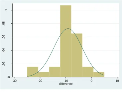
First we need to compute the difference as below:

.generate difference= dass_a_p- b_dass_a

the variable difference is generated now we can check the normality of this variable using histogram.

histogram difference, normal

The following graph will be generated and as shown the distribution is normal.

0

.0

2

.0

4

.0

6

.0

8

.1

D

e

n

sit

y

-30 -20 -10 0 10

difference

(Score difference)

2. Perform STATA using appropriate test.

To perform the paired t test using STATA we need to use the following command:

. t test first variable==second variable

ttest dass_a_p== b_dass_a

See table 5.

(7)

We only need to look for the mean difference, t value, degree of freedom (df), P value (Sig. (2-tailed) and 95% confidence interval

So, the result will be

Mean scoree (sd) before the intervention was 13.34 (5.58)

Mean score (sd) after the intervention was 4.23 (3.19)

Mean score difference (sd) was -9.11 (5.5) with 95% C.I. (-10.52, -7.70) and p value less than 0.001.

So the result will be written as follow:

3. Interpretation and conclusion.

To interpret as follows:

We reject the null hypothesis since P-value is significance (< 0.05) and 95% CI does not cross “0”.

So we accept the alternative hypothesis (HA) which state that there is mean anxiety score difference between before and after intervention.

So the mean anxiety score of after the intervention is smaller than that before by 9.11 scores and it was statistically significant (P value <0.001, 95% CI= (-10.52, -7.70)).

4. Presentation of result.

The final table should be presented as in table 6.

Table 6: Anxiety score after and before intervention among 61 students.

Variables Pre-intervention score mean (SD)

Post- intervention score mean (SD)

Mean score difference (95% CI)

t-statistic (df)

p value

Anxiety score 13.34 (5.58) 4.23 (3.19) -9.11 (-10.91, -7.70) -12.93 (60) <0.001

Conclusion

The above guide will work as an easy step by step guide for a beginner to conduct the analysis using STATA software

Reference