The inductive method and the permanent magnet method for measuring the critical current density in a high-temperature superconducting (HTS) thin film have been investigated numerically. For this purpose, a numerical code has been developed for analyzing the time evolution of the shielding current density in a HTS sample. The results of computations show that, in the inductive method, the critical current density near the film edge cannot be accurately evaluated. On the other hand, it is found that, in the permanent magnet method, even if the magnet is placed near the film edge, the maximum repulsive force is roughly proportional to the critical current density. This means that the critical current density near the film edge can be estimated from the resulting proportionality constants.
c
2010 The Japan Society of Plasma Science and Nuclear Fusion Research
Keywords: current distribution, current measurement, high-temperature superconductor, simulation, thin film DOI: 10.1585/pfr.5.S2113
1. Introduction
High-temperature superconductors (HTSs) can be used in standard applications such as power-transmission cables, flywheel systems and fusion reactor systems. As is well known, HTS materials have various characteristics to keep the superconducting state. In particular, since the crit-ical current densityjCis one of most important parameters characterizing a superconducting property, it is necessary to accurately measure jC.
The standard four probe method is generally used to measure the critical current density jC. In the method, a HTS sample is coated by gold or silver, and subsequently, it should be heat-treated. This process may lead to not only the destruction of the HTS but also the degradation of the HTS characteristics. Therefore, a contactless method has been so far desired for measuringjC.
Claassen et al. proposed a contactless method for measuring the critical current density jC [1]. By apply-ing an ac currentI(t) = I0sin 2πf t to a small coil placed just above a HTS thin film, they monitored a harmonic voltage induced in the coil. From the experimental re-sults, they found that, only when a coil currentI0exceeds a threshold currentIT, the third-harmonic voltage V3 de-velops suddenly. Moreover, it was also revealed that jC can be evaluated from IT. This method is called the in-ductive method and is widely used for the determination of
jC-distributions. On the other hand, Mawatariet al. eluci-dated the inductive method on the basis of the critical state model [2]. As a result, they derived a theoretical formula for the relation between jCandIT.
author’s e-mail: [email protected]
In contrast, Ohshima et al. proposed a novel con-tactless method [3, 4]. While moving a permanent magnet placed above a HTS film, they measure an electromagnetic force acting on the film. As a result, they found that the maximum repulsive forceFMis almost proportional to the critical current density jC. This means that jCcan be esti-mated by measuringFM. This method is called the perma-nent magnet method and is recently used for the measure-ment of the jC-distribution [5].
In order to simulate two types of contactless meth-ods, a numerical code has been developed by analyzing the time evolution of a shielding current density in a HTS thin film [6]. By using the code, we have succeeded in reproducing the contactless methods. However, since we adopt the cylindrical coordinate in the code [6], the center of the coil and magnet is located at just above the origin. Therefore, it is impossible to evaluate a spatial distribution ofjCin a HTS sample by use of the code.
The purpose of the present study is to develop a nu-merical code for analyzing the time evolution of the shield-ing current density in a HTS thin film for the case with the non-axisymmetric model. In addition, we simulate the inductive method and the permanent magnet method by using the code, and investigate the influence of the coil and the magnet position on the determination of the j C-distribution.
2. Governing Equations
In measuring a critical current density jC by means of the contactless methods, a time-dependent magnetic field is applied to a HTS sample. Throughout the present
c
2010 The Japan Society of Plasma
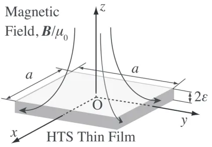
Fig. 1 A schematic view of contactless methods for measuring the critical current densityjC.
study, we assume that a magnetic fieldB/μ0is applied to a square-shaped HTS thin film of the lengthaand the thick-ness 2ε(see Fig. 1). Furthermore, we adopt the Cartesian coordinate systemO :ex,ey,ez, wherez-axis is the thick-ness direction. Note that, in the inductive method, the ori-gin O is chosen at the center of a HTS upper surface. In the permanent magnet method, O is taken at the centroid of a HTS.
As usual, we assume that the thin-layer approxima-tion: since the thickness of the HTS is sufficiency thin, a shielding current density can hardly flow in the thick-ness direction. Hereafter, a HTS film cross-section passing throughz=const. and its boundary are denoted byΩand ∂Ω, respectively.
Under the above assumptions, a shielding current den-sity in a HTS is written as
j=1
ε∇S ×ez, (1)
and the behavior of the scalar functionS(x,t) is governed by the following integro-differential equations [7]:
μ0∂∂
t
Ω
d2xQx−xSx,t+1
εS +∂
∂tB·ez+(∇ ×E)·ez=0. (2)
Here,xis defined byx ≡xex+yey, and is an average operator over the thickness of the HTS. The explicit form ofQ(γ) [7] is
Q(γ)=− 1
4πε2
⎛ ⎜⎜⎜⎜⎜
⎝1γ− γ21+4ε2
⎞ ⎟⎟⎟⎟⎟
⎠. (3)
As is well known, the shielding current density jis closely related to the electric field E. The relation is ex-pressed by theJ-Econstitute equation:
E=E(|j|)j/|j|. (4)
As a functionE(j), we employ the power law [8]:
E(j)=EC(j/jC)16, (5)
Fig. 2 A schematic view of an inductive method.
whereEC is a critical electric field. In the following, we assume that a HTS film has a uniform jC-distribution.
For applying the initial and boundary conditions to (2), we assumeS =0 att =0 andS =0 on∂Ω. By solv-ing the initial-boundary problem of (2), we can obtain the time evolution of a shielding current density. A numerical code has been developed for solving the initial-boundary problem of (2). In order to simulate two types of contact-less methods, the code can be executed by specifying an assumed critical current densityjCand a magnetic fieldB generated by a coil or a permanent magnet.
3. Simulation of Inductive Method
By performing the theoretical calculation based on the critical state model, Mawatariet al. have derived the fol-lowing formula [2]
jNC=F(rmax)IT/ε, (6)
where jN
C is an estimated value of the critical current den-sity jC. F(rmax) is the maximum of a primary coil-factor functionF(r) [2] which can be determined from the config-uration of the coil and the HTS. Furthermore,ITis a lower limit of a coil currentI0 above which the third-harmonic voltageV3begins to develop. For estimatingIT, we use the conventional voltage criterion:V3=0.1 mV⇔I0=IT[2] in the present study.
In the inductive method, the time-dependence mag-netic filed B/μ0 is generated by applying an ac current
I(t) = I0sin 2πf t to an Nc-turn coil placed just above a HTS thin film. For determining the coil position, thexy
coordinates of the center of coil is given by (x,y)=(xc,yc) (see Fig. 2). Furthermore, the cross-section of the coil is expressed asD={(z,r) :|z−Zc| ≤ H/2,|r−Rc| ≤ W/2} with the cylindrical coordinate (r, θ,z). Here, H and W
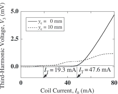
Fig. 3 Dependence of the third-harmonic voltageV3on the coil
currentI0for the case with jC=1 MA/cm2.
6.23×10⁴m−1.
Under the above conditions, let us investigate the in-fluence of the coil position on the determination of thej C-distribution. To this end, they-coordinateycof the center of the coil is changed from 0 mm to 10 mm.
First, for estimating the threshold currentIT, the third-harmonic voltageV3 is calculated as functions of the coil currentI0and is plotted in Fig. 3. We see from this figure that, foryc=0 mm,V3 begins to develop from a certain value ofI0, and after that,V3monotonously increases with
I0. By applying the voltage criterion to theI0-V3 curve foryc =0 mm, we getIT=47.6 mA. By substituting the value ofITto (6), we can obtainjNC =0.99 MA/cm2. This value fairly agrees with the assumed critical current density
jC = 1 MA/cm2. On the other hand, it is found that, for
yc =10 mm, the behavior ofV3 greatly differs inyc=0 mm. According to the voltage criterion, the value ofITis 19.3 mA foryc=10 mm.
Next, let us investigate the relation between the thresh-old currentIT and the critical current density jC. To this end,IT is calculated as functions of jCand is depicted in the inset of Fig. 4. We see from this figure that, foryc=0 mm,ITis roughly proportional to jC. This tendency quan-titatively agrees with Mawatari’s theoretical formula (6). On the other hand, it is found that, foryc=10 mm, the proportional relation betweenITand jCno longer hold.
Finally, let us numerically investigate a limit of the measurement of the critical current densityjC. In order to quantitatively evaluate the accuracy of the threshold cur-rentIT, we define a relative error
εr ≡ ||ITA−ITN||∞/||IAT||∞. (7) Here, INT, a estimated value of IT, is obtained from the voltage criterion, andITA, a theoretical value, is expressed as ITA = jCε/F(rmax). Furthermore, ||f||∞ is denoted by ||f||∞ = Max
jC∈J
|f(jC)|. Here, J is defined by J ≡
Fig. 4 Dependence of the relative errorεr on they-coordinate
yc of the coil. The inset shows that dependence of the
threshold current IT on the critical current density jC.
Here,:yc=0 mm,:yc=10 mm.
{0.1 MA/cm2≤ j
C≤10 MA/cm2}. The relative errorεris calculated as a function ofycand is plotted in Fig. 4. We see from this figure that, foryc>7.5 mm, the accuracy of the inductive method is drastically degraded withyc. An important point is that, foryc=7.5 mm, the sum ofycand the outer radiusRc+W/2 is equal toa/2. From this re-sult, we conclude that, until the outer radius of the coil is equal to the film edge, the critical current density can be accurately evaluated from Mawatari’s theoretical formula.
4. Simulation of Permanent Magnet
Method
In the permanent magnet method, the time-dependence magnetic field B/μ0 is generated by a cylindrical permanent magnet placed above a HTS thin film. Here, the radius and the height of the magnet arerm andhm, respectively, and thexycoordinates of the center of the magnet is denoted by (x,y)=(xm,ym). A distanceL
between a magnet bottom and a film surface is controlled as follows:
(i) From L = Lmax toL = Lmin, the magnet is moved toward the film at the constant speed: v = (Lmax−
Lmin)/τ0. Here,τ0is a constant.
(ii) From L = Lmin toL = Lmax, the magnet is moved away from the film at the same speedv.
Furthermore, for determining the strength of the magnet, we employ a magnetic flux densityBFat (x,y,z)=(0,0, ε) for the case withL = Lmin. Throughout the present sec-tion, the parameters are fixed as follows:a=40 mm, 2ε=
200 nm,xm=0 mm,rm =2.5 mm,hm=3 mm,τ0 =39 s,
Lmax=20 mm,Lmin=0.5 mm,EC=0.1 mV/m,BF=0.3 T. Under the above conditions, we investigate the influ-ence of the magnet position on the determination of the
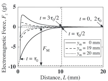
Fig. 5 Dependence of the electromagnetic forceFz on the dis-tanceLfor the case with jC=3.85 MA/cm2.
the center of the magnet is changed from 0 mm to 20 mm. Let us first investigate an electromagnetic forceFz act-ing on the film. For the various values ofym, the electro-magnetic force is calculated as functions of the distance
Land are depicted in Fig. 5. We see from this figure that a repulsive force gradually increases as the magnet moves toward the film (0 ≤ t ≤ τ0). On the other hand, an
at-tractive force decreases to zero when the magnet moves away from the film (τ0 <t ≤ 2τ0). These tendencies do
not change regardless of the magnet position. The elec-tromagnetic force forL=0 can be easily determined by extrapolating theL-Fzcurve (see Fig. 5). In the following, this value is called a maximum repulsive forceFM.
Next, we investigate the relation between the maxi-mum repulsive force FM and the critical current density
jC. Note that the experimental results were obtained for the case with only ym =0 mm [3, 4]. For various values ofym,FMis evaluated as functions of jCand is plotted in Fig. 6. This figure indicates that, forym =0 mm, FM in-creases in proportion to jC. This result is in qualitatively agreement with Ohshima’s experimental one. On the other hand, the results of computations show that, even when the magnet is located atym =19 mm and 20 mm,FM is al-most proportional to jC. In other words, the relation can be expressed as jC=K(xm,ym)(FM/2ε), whereKis a pro-portionality constant.
From this result, we conclude that, even if the mag-net is placed near the film edge, the critical current density
jCcan be determined. Therefore, the jC-distribution in the HTS film can be estimated from the proportionality con-stants determined by the resultingFM-jClines.
5. Conclusion
We have developed a numerical code for analyzing the time evolution of the shielding current density in a HTS sample for the case with the non-axisymmetric model. By using the code, simulating the inductive method and the permanent magnet method, we investigate the influence of
Fig. 6 Dependence of the critical current densityjCon the
max-imum repulsive force FM. Here, : yc = 0 mm, :
ym=19 mm,:ym=20 mm.
the coil and the magnet position on the determination of the distribution of the critical current density jC. Conclusions obtained in the present study are summarized as follows:
(1) In the inductive method, the critical current densityjC near the film edge cannot be accurately measured. In other words, until the outer radius of the coil is equal to the film edge,jCcan be evaluated from Mawatari’s theoretical formula.
(2) In the permanent magnet method, even if the magnet is located near the film edge, the maximum repulsive forceFMis almost proportional to jC. From this re-sult, jCnear the film edge can be estimated from the proportionality constant determined with the resulting
FM−jClines.
Therefore, we conclude that the measurement of jC near the film edge is suitable for the permanent magnet method.
Acknowledgements
This work was supported in part by Japan Society for the Promotion of Science under a Grant-in-Aid for Encour-agement of Scientists No.21920014. A part of this work was also carried out under the Collaboration Research Program at National Institute for Fusion Science (NIFS), Japan. In addition, Numerical computations were carried out on NEC SX-8/8M1 at the LHD Numerical Analysis System of NIFS.
[1] J. H. Claassen, M. E. Reeves and R. J. Soulen, Jr., Rev. Sci. Instrum.62, 996 (1991).
[2] Y. Mawatari, H. Yamasaki and Y. Nakagawa, Appl. Phys. Lett.81, 2424 (2002).
[3] S. Ohshima, K. Takeishi, A. Saito, M. Mukaida, Y. Takano, T. Nakamura, I. Suzuki and M. Yokoo, IEEE Trans. Appl. Supercond.15, 2911 (2005).