23
SIMULATIONS OF FLUID INTERFACES USING CONSERVATIVE
FRONT-TRACKING METHOD FOR 2D EULER SYSTEM
Ullah, M.A.
1*, Khandaker, M.U
2and Mao, D.
31Department of Mathematics, University of Chittagong , Chittagong-4331, Bangladesh. 2
Department of Physics, University of Malaya, 50603 Kuala Lumpur, Malaysia. 3Department of Mathematics, Shanghai University, Shanghai, 200444, P.R. China.
*Corresponding author. E-mail: [email protected], Tel: +88031 726311-14 Ext.4295
ABSTRACT In this paper, we use a conservative front-tracking method for 2D Euler system to do interface simulation. In this method, the movement of fluid interfaces is locally described by 1D Partial Differential Equation (PDE's) derived from the Euler system, and tracking is realized by numerically solving these 1D PDE's in a conservative fashion. We use this method to simulate the Richtmyer-Meshkov instability. Our numerical results are compared with the nonlinear theory developed by Zhang and Sohn (1997) and seem to agree both qualitatively and quantitatively.
(Keyword: Nonlinear growth rate, Conservative front-tracking, Richtmyer-Meshkov instability)
INTRODUCTION
Interfacial instability is an important issue in the research of fluid dynamics nowadays, which attracts numerous attention from physical experiments to numerical simulations. Induced by some physical mechanism, the initially small amplitude perturbations of a fluid interface is eventually grow into big amplitude perturbations. The physical mechanism that induces the instability can be shock passing, which causes Richtmyer-Meshkov instability (RM-instability). This instability was first theoretically studied by Richtmyer in 1960 (Richtmyer R. D., 1960) and experimentally verified by (Meshkov E. E., 1970). The study of interfacial instability has a wide application in sciences and engineering, and the problems that involves to interfacial instabilities are under water explosions, droplet depositions, inertial confinement fusion (ICF), natural phenomena like supernova explosions, etc.
Since the exact solutions to the governing equations for interfacial instability problems, either Euler or Navier-Stokes systems, compressible or incompressible, are hard to find, the results obtained through theoretical study are very limited. Also experimental study of interfacial problems are usually difficult and very expensive, and are often not very accurate in details, especially in the late stages of the flows, due to the imperfectness of experimental conditions. Thus, numerical study of interfacial
problems finds great attention and is expected to give clearer understanding of the problems.
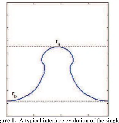
Two types of interfacial instability problems that receive much numerical as well as experimental attentions are the shock-bubble interaction and single-mode instability. In a single-mode RM-instability problem, a shock wave interacts with a sinusoidally perturbed interface between two different fluids in a shock tube. The interaction causes the interface into unstable and small perturbations of this interface grow into nonlinear structures having the forms of bubbles and spikes, (See Figure 1). A spike is a portion of heavy fluid penetrating into light fluid, while a bubble is a portion of light fluid penetrating into heavy fluid. An overall description on the development of RM-instability can be found in literatures (Glimm J. et al.,1998; Holmes R. S. & Sharp D.H., 1995; Holmes R. S. et al., 1999; Holmes R.S., 1994; Li X. L. & Zhang, 1997; Zhang Q. & Sohn S-I., 1996; Zhang Q. & Sohn S-I., 1997; Zhang Q. & Sohn S-I., 1999). Furthermore, a detailed review on the theoretical, experimental and numerical developments of RM-instability is available in (Benjamin et al.,1993).
24
Figure 1. A typical interface evolution of the
single-mode RM-instability with tip of bubble
r
band tip spike
r
s.The fundamental quantities of interest for investigation of the RM-instability are the amplitude and amplitude growth rate of the perturbation on the interface. The amplitude
a
(
t
)
is defined as one-half of the vertical distance between the tips of spike and bubble,
(
)
2
1
)
(
t
r
sr
ba
… … … (1.1)where
r
s andr
b are the positions of the spike andbubble tips, as shown in Figure 1. The amplitude growth rate is defined as the derivative of the amplitude
a
(
t
)
with respect tot
, which turns out to be
(
)
2
1
)
(
t
v
sv
ba
… … … (1.2)where
v
s andv
b are the velocities of the spike andbubble tips.
Zhang and Sohn developed a quantitative nonlinear theory for the compressible RM-instability in both two and three dimensions [18-20]. Their theoretical predictions was based on pade approximation and constructed the perturbation amplitude and amplitude growth rate. Their analytical predictions were also in good agreement with the experimental results as well as nonlinear numerical simulations. They also obtained distinct bubble and spike velocities, and the overall growth rate at the interface valid for both early and late times. Linear and nonlinear theory are also discussed in (Nishihara et al., 2010).
In this paper, we use the conservative front-tracking method developed by Mao to numerically simulate (Benjamin R., et al.,1993) single-mode instability problems. For the single-mode RM-instability problem, we compute the amplitudes and amplitude growth rates. In this work, the computed perturbation amplitudes and amplitude growth rates are compared with the nonlinear analytical results obtained by Zhang and Sohn[18-20]. However, our numerical results qualitatively in good agreement with the analytical nonlinear results. The paper is organized in the following way: In section 2, briefly describe Mao's conservative front-tracking method. Section 3, gives the numerical example. Finally, section 4 gives the conclusions.
NUMERICAL METHOD
In this section, we are going to give a brief description of the mathematical formulation of Euler system, material interface for multifluid and the conservative front-tracking method that is to be used for the simulation. The method was designed for general 2D conservation laws and tracked both the shocks, contact discontinuities and material interfaces.
Two-Dimensional Euler System of Fluid dynamics
We thus consider the 2D hyperbolic conservation laws of the form:
u
t
f
(
u
)
x
g
(
u
)
y
0
… … … (2.1)
u
(
,
u
,
v
,
E
)
T … … …(2.2a)
f
(
u
)
(
u
,
u
2,
uv
,
(
E
p
)
u
)
T … … … (2.2b)
g
(
u
)
(
v
,
uv
,
v
2,
(
E
p
)
v
)
T … … …(2.2c)where
denotes the density,u
andv
are the particle velocities in the x- and y-directions,p
is thepressure and
E
the total energy. The term
u
is the x-component of momentum, and the term
v
is the y-component of momentum. The total energy can be defined as,
(
)
2
1
2 2v
u
E
… … … (2.2d)where
(
)
2
1
2 2v
u
E
is the kinetic energy and25 which is related to the fluid components of interest, and is assumed to satisfy the equation of state of the form
p
(
1
)
… … … (2.2e) where
is the specific ratio of heats. We use Eqs. (2.2a)-(2.2c) with equation of state (2.2e) as governing equations for our computation. It is well known that the solution to (2.1) may develop discontinuities, shocks, contact discontinuities and slip lines, no matter how smoothly the initial and boundary conditions are proposed.Two-fluid Flows and Material Interfaces
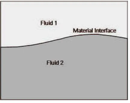
Here, we consider two-fluid flow in two space dimensions, i.e. a flow involves two different fluids which are separated by a well-defined interface, called material interface. Two fluid components will not be mixed with each other in the flow. Therefore, the entire flow region can be viewed as constitution of two regions, in each of which flows only one fluid. The situation is shown in Figure 2. The two-fluid flow is the simplest case of multifluid flow, in which more than one fluids are involved and the different fluids are separated by well-defined interfaces.
Figure 2. In two fluid flow, the fluid 1 and fluid 2 are separated by a well-defined material interface.
The flow in each region is described by the Euler system (2.1) with the corresponding EOS of the fluid in the region. We assume that the two fluids are both of the ideal gases with the EOS's as
p
(
1
1
)
… … … (2.3a)
p
(
2
1
)
… … … (2.3b)where
1 and
2 are the ratios of specific heats of the individual components, respectively. The material interface that separates the two fluids is also alinearly degenerated discontinuity i.e. it coincides with the contact discontinuity and slip line and moves with the fluids. Therefore, the normal velocity and pressure of the flow are continuous across the interface, and the density, tangential velocity and ratio of specific heats in the EOS may jump. As we already mentioned, the material interfaces are very unstable in two-fluid flows; small perturbations on the interfaces will be greatly amplified by some physical mechanism. The physical mechanism that induces the instability can be shock passing, which causes Richtmyer-Meshkov instability, gravity, which causes Rayleigh-Taylor instability, or velocity shear, which causes Kelvin-Helmholtz instability. In this study, we are going to present the numerical simulations of important example of interfacial instabilities, i.e. Benjamin's single-mode RM-instability experiments.
Conservative Front-Tracking Method
In the last decade, Mao developed a front-tracking method for the 2D Euler system, (Mao De-kang, 2000; Mao De-kang, 2007). Like all the front-tracking methods, say (Glimm J. et al.,1998; Holmes R. S, 1995; Holmes R.S, 1994; Li X. L. & Zhang Q., 1997), it is almost free of numerical dissipation. However, the following two features distinguish it from the other front-tracking methods: 1) The discontinuity curves are tracked by enforcing the conservation properties of the Euler system rather than the propagation speeds obtained by solving Riemann problems on the curve. 2) The movement of discontinuity curves is locally described by 1D PDE's derived from the Euler system, and the tracking is realized by locally discretizing these 1D PDE's on Cartesian sub-grid. Designed in such a way, Mao's front-tracking method is much simpler than the other front-tracking methods, it runs on Cartesian grid and uses no adaptive grid. More important, it is conservative. The method has already been successfully implemented on various numerical experiments and shows its efficiency and effectiveness in 1D and 2D cases, see (Mao De-kang, 2000; Mao De-De-kang, 2007; Ullah M.A., 2011; Ullah M.A., Wenbin G & Mao De-kang, 2011; Ullah M.A. et al., 2010).
NUMERICAL EXAMPLE
26 right to left of the shock tube and collided with the
sinusoidal interface with
SF
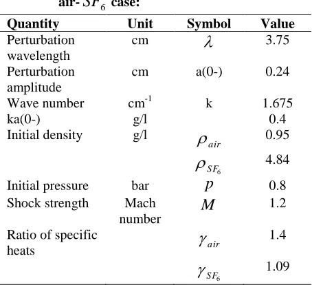
6 and then interfacestarts to move. The rectangular domain is taken long enough in the horizontal direction so that there is no influence from the two ends on the measurements of the interfaces during the computational time. Flow through boundary conditions are imposed on the right and left, periodic boundary conditions are imposed on the top and bottom sides of the tube. The shock reflects and refracts when passing the interface and produces a reflected and transmitted shock, see in (Holmes R. S. ET AL, 1999). The initial set-up is shown in Figure 3 and the parameters are taken from Benjamin's experiments which is shown in Table 1:
Figure 3. Initial set-up of the single-mode
RM-instability for air-
SF
6.Table 1: Experimental parameters for
air-
SF
6 case:Quantity Unit Symbol Value
Perturbation wavelength
cm
3.75Perturbation amplitude
cm a(0-) 0.24
Wave number cm-1 k 1.675
ka(0-) g/l 0.4
Initial density g/l
air
0.956 SF
4.84Initial pressure bar
p
0.8 Shock strength Machnumber
M
1.2Ratio of specific
heats
air1.4
6 SF
1.09QUALITATIVE AND QUANTITATIVE DISCUSSIONS
In this section we present the qualitative and quantitative predictions of our numerical results for overall amplitude, amplitude growth rate and the growth rates of the spike and bubble, and compare the results with nonlinear theory predicted by Zhang and Sohn (Zhang Q. & Sohn S-I, 1997 ; Zhang Q. & Sohn S-I, 1996).
Figure 4 shows the amplitudes and amplitude growth rates given by impulsive model, the numerical solution of linear theory, the nonlinear theory obtained by Zhang and Sohn, the numerical simulation with our conservative front-tracking method and the experiments. The amplitude and amplitude growth rates are computed using (1.1) and (1.2), respectively. The data for the impulsive model, the linear theory, the nonlinear theory by Zhang and Sohn and the experiments are picked from (Zhang Q. & Sohn S-I, 1997).
In Figure 4, we compare our computed perturbation amplitude and amplitude growth rates with the nonlinear theory, nonlinear theory by Zhang and Sohn (Zhang Q. & Sohn S-I, 1997) and Richtmyer's
impulsive model for air-
SF
6 case. Figure 4(a) shows the prediction of the amplitude, while figure 4(b) express the growth rates. In both figures our numerical solutions are qualitatively and quantitatively in good agreement with those of nonlinear theory. The similarity in structure of the two growth rates curves, ours and Zhang and Sohn's in Figure 4, indicated that compressibility and nonlinear effects is also qualitatively well captured in our simulation.The growth rate determined from the experimental data was 9.2 m/sec over the time period 310-750
sec
. Using the least square method, we compute the growth rate of our conservative front tracking method over the same experimental period (310sec
27
(a)
(b)
Figure 4. Numerical simulations are compared with nonlinear theory by Zhang and Sohn, linear theory, impulsive model and experiments: (a) amplitude and (b) growth rate.
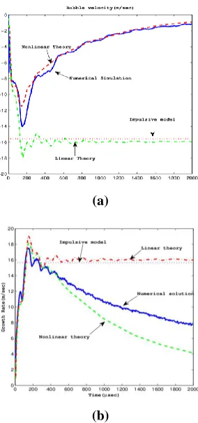
Potential flow model describes the amplitude growth rate through the late-time, nonlinear regime by the spike and bubble velocity evolution. Layzer (1955) first studied single-mode potential flow model to compute the bubble velocity for Rayleigh-Taylor case. (Hecht et al, 1994) extended Layzer-type model and studied the bubble velocity for RM-instability corresponding to an Atwood number A=1, which shows the decay of bubble velocity. Their model was applied to two-dimensional single-mode bubble evolution as well as two-bubble competition. Zhang and Sohn also compared their nonlinear theory with that of potential model (Holmes R.S.,1994; Li X. L. & Zhang Q., 1997; Mao De-kang, 2000).
(a)
(b)
Figure 5. Numerical simulation with our results compare with nonlinear solution by Zhang and Sohn, linear theory, impulsive model and experimental time (a) Bubble velocity and (b) Spike velocity.
28
CONCLUSION
We have numerically simulate Benjamin’s air-SF6 experiment of RM-instability and compared our results with those of Zhang and Sohn’s analytical predictions with the perturbation amplitude and amplitude growth rate. With this comparison, we can predict that our simulations are also in good agreement with the nonlinear theory. This shows that our conservative front-tracking method is efficient and effective for simulations of material interface.
REFERENCES
Benjamin R., Besnard D. and Haas J. F.(1993). Shock and reshock of an unstable interface. LANL report, LA-UR 92-1185.
Brouillette M. (2002). The Richtmyer-Meshkov instability. Annu. Rev. Fluid Mech. 34: 445-468.
Glimm J., Graham M. J., Grove J., Li X. L., Smith T. M., Tan D., Tangerman F. and Zhang Q.(1998). Front tracking in two and three Dimensions, Computers Math. Applic 35(7): 1-11.
Hecht J., Alon U., and Shvarts D.(1994). Potential flow model of Rayleigh-Taylor and Richtmyer-Meshkov bubble fronts. Phys. Fluids 6(12): 4019-4030.
Holmes R. S., Grove J. W. and Sharp D. H. (1995). Numerical investigation of Richtmyer-Meshkov instability using front-tracking. J. Fluid Mech. 301: 51-64.
Holmes R.S. et al. (1999). Richtmyer-Meshkov instability growth: experiment, simulation and theory. J. Fluid Mech. 389: 55-79.
Holmes R.S.(1994). A numerical investigation of the Richtmyer-Meshkov instability using front–tracking. Doctor's dissertation, State University of New York at Stony Broke.
Li X. L. and Zhang Q.(1997). A comparative numerical study of the Richtmyer- Meshkov instability with nonlinear analysis in two and three dimensions. Phys. Fluids 9(10): 3069-3077.
Mao De-kang (2000). Towards front tracking based on conservation in two space dimensions. SIAM. J. Sci. Comput. 22(1): 113-151.
Mao De-kang (2007). Towards front-tracking based on conservation in two space dimensionsII, tracking discontinuities in capturing fashion. J. Comput. Phys. 226:1550-1588.
Meshkov E. E.(1970). Instability of a shock wave accelerated interface between two gases. NASA Tech. Trans F-13: 074.
Nishihara K., Wouchuk J. G., Matsuoka C., Ishizaki R. and Zhakhovsky V.V. (2010). Richtmyer-Meshkov Instability: theory of linear and nonlinear evolution. Phil. Trans. R. Soc. A. 368: 1769-1807.
Richtmyer R. D. (1960). Taylor instability in shock acceleration of compressible fluids. Commun. Pure Appl. Math.13: 297-319.
Ullah M.A. (2011). Numerical Simulations of Material Interfaces Using Conservative Front Tracking Method. Doctor's dissertation, Shanghai University, Shanghai, China.
Ullah M.A., Wenbin G and Mao De-kang (2011). Numerical simulations of Richtmyer-Meshkov instability using conservative front-tracking method. Appl. Math. Mech. (English Edition) 32(1):119-132.
Ullah M.A., Wenbin G. and Mao De-kang (2010). Numerical Simulation of a single-Mode Richtmyer-Meshkov Instability using Conservative Front Tracking Method. Vietnam Journal of Mathematics 38(3): 323-339.
Wenbin G., Ullah M. A. and Mao De-kang (2010). Conservative Front Tracking Method of Multimaterial Interfaces. Comm. on Appl. Math. and Comput. 24(1): 61-69.
Zhang Q. and Sohn S-I. (1997). Nonlinear theory of unstable fluid mixing driven by shock wave. Phys. Fluids. 9(4):1106-1124.
Zhang Q. and Sohn S-I. (1999). Quantitative theory of Richtmyer-Meshkov instability in three dimension. ZAMP 50:1-46.