Parameter Estimation for Bivariate Mixed Lognormal Distribution

(1)

41

Parameter Estimation for Bivariate

Mixed Lognormal Distribution

Ching Yee Kong*_{, Suhaila Jamaludin, Fadhilah Yusof, Hui Mean Foo}

*_{Department of Mathematics, Faculty of Science,}

Universiti Teknologi Malaysia, 81310, Skudai, Johor, Malaysia.

*_{Corresponding email: [email protected]}

Abstract

Bivariate mixed lognormal distribution is a probability model used for representing rainfalls behavior at two monitoring stations. The paper discuss on the parameter estimation for bivariate mixed lognormal distribution in which all parameters are assumed to be unknown. Six cases were considered in the analysis and the parameters were estimated using the maximum likelihood. The optimal model was selected based on the minimum Akaike’s information criterion (AIC) from selected model. The analysis is run by using the rainfall data observed for the time period of 33 years (1975-2007) from Arau, Perlis with each of the other 7 nearby monitoring stations and 5 far distance stations. Among the 7 stations studied, 6 stations (87.5%) choose the same case model (M2) as the minimum AIC procedures. Meanwhile, 4 of the far distance stations choose the case M2 as the best fit case model.

(2)

1. INTRODUCTION

Rainfall data is widely used in hydrological application, therefore many researches had carried out to estimate the characteristic of rain (Moron et al., Young, Zhang and Singh, Mielke et al., Habib and Krajewski[1]-[5]). The rainfall behaviour of two monitoring stations usually recognise bivariate mixed lognormal distribution as a suitable probability model. The concept of applying mixed distribution in rainfall data origin by Kedem[6] while Shimizu[7] enriched the usage of mixed distribution by implementing it in bivariate distribution. Mixed distribution is a mixture of discrete distribution and continuous distribution. The rainfall characteristic is a combination of discrete distribution and continuous distribution where discrete distribution represents the zero values for the days that do not rain and continuous distribution represents rainfall amount on rainy days. The main objective of this paper is to estimate all the parameters of bivariate mixed lognormal distribution where all the parameters are assume to be unknown. The past research that have been carried out in Malaysia mostly do not considered the attribute of the rainfall which there exist zeros value (days that do not have rain). The important of included the zeros for the study of characterization of rainfall can be analyzed as suggested in Ha and Yoo [8].

2. RAINFALL DATA

(3)

43

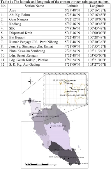
Table 1: The latitude and longitude of the chosen thirteen rain gauge stations.

No. Station Name Latitude Longitude

Arau 6o25’48”N 100o16’12”E

1. Abi Kg. Bahru 6o28’48”N 100o16’48”E 2. Guar Nangka 6o22’12”N 100o18’00”E

3. Kodiang 6o30’36”N 100o10’48”E

4. SIK 5o48’36”N 100o43’48”E

5. Dispensari Kroh 5o42’36”N 101o00’00”E

6. Bkt Berapit 5o22’48”N 100o28’48”E

7. Rumah Penjaga JPS. Parit Nibong 5o07’48”N 100o30’36”E 8. Jam. Sg. Simpangn ,Jln. Empat 4o21’00”N 101o55’12”E 9. Pintu Kawalan Sembrong 2o26’24”N 102o11’24”E 10. Ldg. Benut ,Rengam 1o52’48”N 103o03’00”E 11. Ldg. Getah Kukup , Pontian 1o50’24”N 103o21’00”E 12. S. K. Kg. Aur Gading 1o21’00”N 103o27’36”E

(4)

3. METHODOLOGY

The steps to estimate the parameter for bivariate mixed lognormal distribution is first defined by Shimizu [7] and applied in this study. The rainfall data of two selected rain gauge station will be restructured. The maximum likelihood estimation (MLE) equations of the parameters are calculated according to six cases model which are considered. The optimal model is selected based on the minimum Akaike’s information criterion (AIC) from the six case models.

3.1 Restructure Rainfall Data at Two Stations

The rainfall data of two stations can be categorized into dataset in types of

 

0,0 ,

 

_x,0 _,



₀_,_y



_and

 

_x_,_y _where_x_,_y_,_x_and_y_{are positive values. Under homogeneous}

assumption in time, the sample size N can be reconstructed into the four types of dataset without loss of generality

0

n n1 n2 n3

0 , ,

0_  

1 , ,

1 xn

x  0,,0 x1,,xn3

0 , ,

0_ 0,_,0  

2 , ,

1 yn

y _ y1,,yn3

where



_r nr N

3

0 ,xi 0



i1,,n1



 _,





2

, , 1

0 j n

yj   

 _,





3

, , 1 0

,y k n

(5)

45

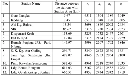
Table 2: Distance between the twelve stations with Station Arau and the values of



r0,1,2,3



nr

No. Station Name Distance between the stations with Station Arau (km)

0

n n1 n2 n3

1. Guar Nangka 5.67 6511 1304 1189 3049

2. Kodiang 7.45 6510 1048 1190 3305

3. Abi Kg. Bahru 13.34 5698 1869 2002 2484

4. SIK 85.67 5316 1730 2384 2623

5. Dispensari Kroh 113.69 5253 1752 2447 2601

6. Bkt Berapit 119.04 5315 2124 2385 2229

7. Rumah Penjaga JPS. Parit

Nibong 146.97 5998 2507 1702 1846

8. S. K. Kg. Aur Gading 294.71 5340 2672 2360 1681 9. Jam. Sg. Simpangn ,Jln.

Empat

492.07 4846 2253 2854 2100

10. Pintu Kawalan Sembrong 592.43 4961 2318 2740 2035 11. Ldg. Benut ,Rengam 614.03 5167 2371 2532 1982 12. Ldg. Getah Kukup , Pontian 666.51 4858 2434 2842 1919

3.2 Bivariate Model for Rainfall Data

Let



X,Y



be the random vector of rainfall values at two rain gauge station, where the probability distribution satisfies



X 0,Y 0



0 P



0X x,Y 0



 ₁F

 

x , x0

P 



X 0,0Yy



 ₂G

 

y , y0

P 



0X x,0Y y



 ₃H

 

x,y , x,y0

P  (1)

where0_r1(r0,1,2,3)and ₀₁₂₃1, Fand Gare univariate positive continuous distribution functions, and H is a bivariate positive continuous joint distribution function. The conditional on rainfall at both of two stations or either one station are



X x|0X x,Y 0



F

 

x x0

P



Y y|X 0,0Y  y



G

 

x y0

P



X x,Y y|X 0,Y 0



H

 

x,y x,y0

P (2)

3.3 Six Cases for Parameter Estimation

(6)

M1: 2 2 2 2 2 1 2 1 2 2 1

1  ,   ,   ,  

       

M2: 2

2 2 2 2 1 2 1 2 2 1

1  ,   ,   ,  

       

M3: 2 2

2 2 2 2 1 2 1 2 2 1

1  ,   ,     

         

M4: 2

2 2 2 2 1 2 1 2 2 1

1  ,   ,   ,  

       

M5: 2 2

2 2 2 2 1 2 1 2 2 1

1  ,   ,     

         

M6: 2

2 2 2 2 1 2 1 2 2 1

1  ,   ,   ,  

        ₍₃₎

These six cases are considered because the shape parameter  affects the structural stability in a lognormal distribution.

4. RESULT AND DISCUSSION

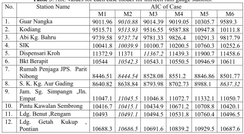
The results of AIC values of each cases model are displayed in Table 3 with the bolded and italic values indicated the lowest AIC values. Case M2 is the dominated best fitted case model among other case models. Among the seven nearby stations, six of the stations chose case M2 and only one station chose case M3. While for the five stations that located far from Arau station, four stations attained the lowest AIC values for case M2 and one station attained case M6 as the lowest AIC values.

(7)

47

Table 3: AIC values for each case model for thirteen rain gauge stations.

No. Station Name AIC of Case

M1 M2 M3 M4 M5 M6 1. Guar Nangka 9011.96 9010.88 9014.39 9019.05 10305.7 9589.3 2. Kodiang 9515.71 9513.93 9516.55 9587.88 10947.8 10111.8 3. Abi Kg. Bahru 9739.58 9737.74 9781.33 9826.4 10291.3 9817.79 4. SIK 10041.8 10039.9 10100.7 10200.5 10760.3 10252.6 5. Dispensari Kroh 11372.9 11371 11367.2 11439.3 11900.7 11458.6 6. Bkt Berapit 10544 10542.3 10543.1 10550.5 10946.9 10611 7. Rumah Penjaga JPS. Parit

Nibong 8446.51 8444.54 8528.08 8551.2 8846.86 8501.77 8. S. K. Kg. Aur Gading 8640.82 8638.84 8793.98 8702.73 8988.1 8637.32

9. Jam. Sg. Simpangn ,Jln.

Empat 11047.1 11045.5 11046.8 11072.7 11332.1 11050.7 10. Pintu Kawalan Sembrong 10416.7 10415.1 10434.9 10671.2 10708.8 10420.1 11. Ldg. Benut ,Rengam 10493 10491.1 10494.5 10531.8 10760.4 10496.5 12. Ldg. Getah Kukup ,

Pontian 10688.3 10686.5 10691.6 10839.2 10929.5 10687.6

5. CONCLUSIONS

The characteristic of rainfall is a mixed distribution which contain discrete distribution (days that do not rain) and continuous distribution (days that rain). It is prominent to analyze the rainfall data by including the zero values. The estimated parameters of bivariate mixed lognormal distribution were determined by the minimum value of AIC values. In this study, six of the seven nearby stations and four of the five far located stations of station Arau have chosen case M2 based on the minimum AIC procedures. The parameter estimated will be further used for the effect of zero measurements.

Acknowledgment

(8)

REFERENCES

[1] Moron, V.; Robertson , A.W.; and Ward, M.N. (2006). Seasonal Predictability and Spatial Coherence of Rainfall Characteristics in the Tropical Setting of Senegal.Monthly Weather Review. 134(11): 3248-3262.

[2] Young, K.C. (1992). A Three-Way Model for Interpolating for Monthly Precipitation Values. Monthly Weather Review. 120(11): 2561-2569.

[3] Zhang, L. and . Singh, V.P (2007). Bivariate rainfall frequency distributions using Archimedean copulas. Journal of Hydrology. 332(1-2): 93-109.

[4] Mielke, P.W.; Williams, J.S.; and Wu, S.C. (1977). Covariance Analysis Technique Based on Bivariate Log-Normal Distribution with Weather Modification Applications. Journal of Applied Meteorology. 16(2): 183-187.

[5] Habib, E. and Krajewski, W.F. (2001). Estimation of Rainfall Interstation Correlation. Journal of Hydrometeorology. 2: 621-629.

[6] Kedem, B.; Chiu, L.S.; and North, G.R. (1990). Estimation of Mean Rain Rate' Application to Satellite Observations. Journal of Geophysical Research. 95(D2): 1965-1972.

[7] Shimizu, K. (1993). A Bivariate Mixed Lognormal Distribution with an Analysis of Rainfall Data. Journal of Applied Meteorology. 32(2): 161-171.

[8] Ha, E. and Yoo, C. (2007). Use of mixed bivariate distribution for deriving inter-station correlation coefficients of rain rate. Hydrological Processes. 21(22): 3078-3086.