R E S E A R C H
Open Access
Realistic modeling of a combined heat
and power plant in the context of mixed
integer linear programming
Thomas Weber
*, Nina Strobel, Thomas Kohne, Jakob Wolber and Eberhard Abele
FromThe 7th DACH+ Conference on Energy Informatics Oldenburg, Germany. 11-12 October 2018
* Correspondence: [email protected] Institut für
Produktionsmanagement, Technologie und
Werkzeugmaschinen, TU Darmstadt, Otto-Berndt-Straße 2, 64287 Darmstadt, Germany
Abstract
In addition to renewable energy sources, the transition of the German energy system will increasingly involve the use of decentralized combined heat and power plants (CHP). In order to use this promising technology cost-optimally, modeling approaches must be developed that enable optimization of the systems. Mixed integer linear programming (MILP) is a powerful tool for solving mathematical optimization problems. However, to reduce the computing time the model formulation requires compelling simplifications in relation to reality. The aim of this paper is to present a modeling approach for a combined heat and power plant that depicts dynamic power changes more accurately than existing approaches. Power gradients are mapped by differentiating between the control signal of the CHP unit and the actually generated power output for thermal and electrical power. Finally, the accuracy of the modeling approach is examined in a field test and evaluated according to the accuracy achieved.
Keywords: CHP, MILP, Validation
Introduction
Energy supply in Germany is increasingly changing from a centralized to a decen-tralized generation structure (Strasser et al. 2015; Goldthau 2014). Especially the use of decentralized combined heat and power plants (CHP) is increasing, as it al-lows high fuel utilization rates to be achieved. However, since in addition to electri-city generation, heat generation must be considered, the forward-looking operation of the plants is more complex than in case of separate generation of electricity and heat. The mixed integer linear programming is to be emphasized in the so called unit commitment problem and also used in this work (Poler et al. 2014). Existing modeling approaches of CHP units in the context of mathematical optimization show great cost saving potential. However, due to model simplifications and as-sumptions, the resulting plant schedules are not directly applicable in many cases. Within the scope of this work, existing approaches for the mathematical modeling
of CHP are presented and further developed regarding their applicability. Therefore, the presented approach is validated by a field test with a real CHP system.
Literature review
There are already many approaches in the literature to solve the so-called economic dispatch problem (Boji_C and Stojanovi_C1996; Silvente and Papageorgiou2017; Wang et al.2015; Christidis et al.2012; Costa and Fichera2014; Spieker2013; Steck2012; Steen et al.2015; Fubara et al.2014; Arroyo and Conejo2000; Carrion and Arroyo2006; Mitra et al. 2013; Bosman et al.n.d.; Bosman2012). In many cases these have already been applied to cogeneration plants (Boji_C and Stojanovi_C1996; Silvente and Papageorgiou2017; Wang et al.2015; Christidis et al.2012; Costa and Fichera2014; Spieker2013; Steck2012; Mitra et al. 2013; Bosman et al. n.d.; Bosman2012). Power gradient restrictions in the context of economic dispatch are usually implemented by limiting the change in the set power be-tween two time stepsPt= 2−Pt= 1≤ΔPmax(Wang et al.2015; Steck2012; Arroyo and
Con-ejo 2000; Carrion and Arroyo2006; Mitra et al.2013). The forecasted generated and thus marketed powerPavailableis equated with the set powerPset, although due to the inertia of the systems there are sometimes significant differences between these two. For example, if the operating point of a plant is increased from 80% (time step 1) to 100% (time step 2) in a system with a maximum power gradient of 20%, a marketable output of 100% is assumed in previous work for time step 2. However, assuming a linear power increase, the actual aver-age power output in time step 2 will be only 90%. Only Bosman et al. take the changed power output into account (Bosman et al. n.d.; Bosman 2012), however, operation of the CHP unit in partial load is excluded, which is an enormous limitation of the approach. This work presents an approach to consider the effect of power gradients on the actual power output also in partial load operation for both electrical and thermal. The approach is then validated with the work of Steck et al. (Steck2012) with regard to realism, since the some of the here presented model structure is close to Stecks‘work.
Model
The optimization model provides a cost-optimized operating strategy for a CHP in com-bination with a thermal storage. Due to external influences (e.g. electricity price, heat load), different power states are optimal at different times. Therefore, a time step widthΔt
is selected, with which the observation time frame is divided intottotal
Δt ¼T in total. The
de-cision variables used in the model are listed in Table 1. The main task of the CHP is to cover the required heat load. In addition to providing heat, the CHP unit can sell the elec-tricity generated on the power exchange at an elecelec-tricity price that changes every 15 min.
In advance, heat loadQ_demandt and electricity pricecelec
t are assumed to be known.
Objective function
The objective function in eq.1is based on the PhD thesis of Steck.
c¼XT
t¼1 −P
available
t ∙celect þδ start−up
t ∙cstart−upþP fuel t ∙cfuel
ð1Þ
Parameters
Electricity prices [Euro = kWh]:celec t
Fuel cost [Euro = kWh]:cfuel
Costs caused by increased machine wear during switching operations [Euro]:cstart−up
Electrical: Max/min electrical power [kW]:Pmax/Pmin
Overall efficiency of the CHP:ηtotal
Electrical efficiency whilePsett ;elec¼Pmax=Pmin:ηelec;max=ηelec;min
Maximum power gradient for power increase/ reduction in operating mode:ΔPmax/
ΔPmin
Maximum power gradient when switching between off and on:ΔPmax,start−up
Energy shortage during start-up because of the inertia of the CHP:Pstart−up
Thermal: Heat demand [kW]:Q_demandt
Thermal inertia of the CHP: g
Maximum state of charge of the thermal storage [kWh]:Emax
Thermal losses of the thermal storage [kWh] between two periods, when idle:QLoss1
Percentage of the state of charge, that will be lost between two periods:q_Loss2
Max charging/discharging power [kW]:Q_charge;max/Q_discharge;max
Efficiency during charge/discharge:ηcharge/ηdischarge
Operating state
Equation2limits the permissible electrical output power of the CHP.
Pmin∙δont ≤Psett ;elec≤Pmax∙δont ∀t ð2Þ
The electrical output power can only be either at zero or between Pmin and Pmax. (Steck2012)
Power-dependent efficiency
Steck proposes to define the fuel consumption as a function of the operating state and the current electrical output (eq. 3). Factors c and k are defined via efficiency
ηelec, min
and ηelec, max in minimum load point Pmin and maximum load point Pmax (See (Steck 2012) page 34).
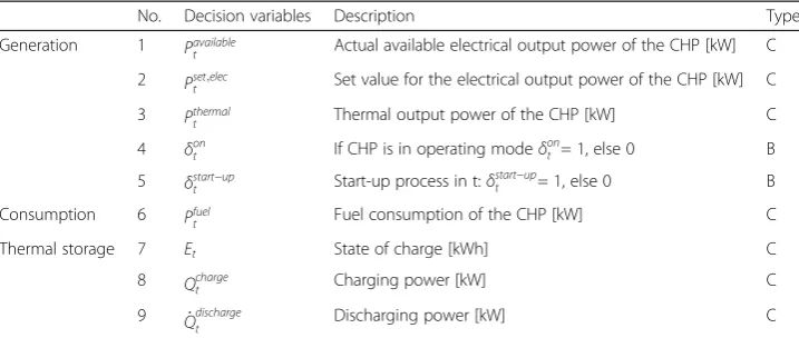
Table 1Decision variables. Index t: Current time step.
No. Decision variables Description Type
Generation 1 Pavailable
t Actual available electrical output power of the CHP [kW] C
2 Pset;elect Set value for the electrical output power of the CHP [kW] C
3 Pthermal
t Thermal output power of the CHP [kW] C
4 δont If CHP is in operating modeδont = 1, else 0 B
5 δstart−upt Start-up process in t:δstart−upt = 1, else 0 B
Consumption 6 Pfuelt Fuel consumption of the CHP [kW] C
Thermal storage 7 Et State of charge [kWh] C
8 Qcharge
t Charging power [kW] C
9 Q_discharge
t Discharging power [kW] C
Pfuelt ¼c∙δont þk∙Psett ;elec ∀t ð3Þ
In contrast to the assumption of constant efficiency, this approach provides incen-tives for operation with more favourable efficiency. (Steck2012)
Cogeneration
In eq. 4, a relation between electrical power and heat generation is established. Steck assumes that the overall efficiency ηtotal is constant, while the electrical efficiency is variable over the load range. This results in a relatively high heat generation with rela-tively low electrical power generation at the minimum load point. (For f1 and f2 see (Steck2012) page 35.)
Pthermalt ¼ f1∙Psett ;elecþf2∙δont ∀t ð4Þ
Start-up
A start-up of the CHP is indicated by the variableδstartt −up. Equation5forcesδstartt −upto
one if the CHP switches on at the beginning of time step t. (Steck2012)
δstart−up t ≥δont −δ
on
t−1 ∀t ð5Þ
Power gradient constraints
An extension to the state of the art CHP model is offered by the following system of constraints to consider the inertia of the system with its power gradients. State of the art approaches (Wang et al. 2015; Steck 2012; Arroyo and Conejo 2000; Carrion and Arroyo 2006; Mitra et al. 2013) limit the power change between two time steps by equation 6. In addition to the positive power gradient constraint in 6, our model introduces a negative power gradient constraint in equation 7. But even with these two constraints, jumps or leaps in power are not prevented.
Psett −Ptset−1;elec≤ΔPmaxþδtstart−up∙ðΔPstart−up−ΔPmaxÞ ∀t ð6Þ
Ptset;elec−Ptset−1;elec≥ΔPmin ∀t ð7Þ
Here, in addition to the set powerPsett ;elec, a new continuous variablePavailablet is
intro-duced that determines the actual available electrical power output of the CHP unit.
Equation8shows the relationship betweenPsett ;elecandPavailable
t .
Pavailable t ¼P
set;elec
t þδstartt −upΔPstart−upBþ P
set;elec t−1 −P
set;elec t
Δ Pmax−Pmin
2ΔPmaxþΔPminA ∀t ð8Þ
triangle, illustrated in Fig. 1. To meet the linearity condition, an edge of the error triangle is assumed to be constant. With taking12ðΔPmaxþΔPminÞas a length for the constant edge, a good approximation can be achieved. B, on the other hand, de-scribes the energy shortage that occurs because of the inertia when the system starts up, including reaction and start-up time. The energy shortage Pstart−up associated with starting up the CHP plant is determined from historical data. Although the
average available powerPavailable
t is calculated,P set;elec
t informs the user directly about
the set values for the CHP unit.
Thermal balance
The heat generated is either stored or passed directly to the consumer. Accordingly, the heat demand can be met both directly by the CHP unit and by the thermal stor-age unit. As in (Steck 2012; Steen et al.2015) our approach models a thermal grid with a thermal storage. In our approach though, the inertia of the CHP can be mod-elled with the factor g. In the thermal balance (equation9), a proportion of the ther-mal power is shifted into the next time step.
−Q_demandt þηdischarge∙Q_discharget −Q_charget þg∙Pthermalt þð1−gÞ∙Ptthermal−1 ¼0 ∀t ð9Þ
In addition the separate balance for the heat storage in equation 10 is required to model the charging and discharging process.
Et∙q_Loss2þΔt ηcharge∙Q_ charge t −Q_
discharge
t ∙ηdischarge
−QLoss1¼Etþ1 ∀t ð10Þ
As in (Steen et al. 2015) the following losses can be modelled: For sensitive thermal storages charge-dependent losses are modelled by q_Loss2 . Continuous
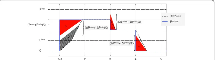
Fig. 1Power gradient energy correction. The figure shows the set valuesPset,elecfor an exemplary run of a CHP
unit. The graphPCHP,outputdisplays the reaction of the CHP unit to the given set values, under the assumption
that it behaves linearly. The red triangles illustrate the Term A in equation8. Term A aims to approximate the area between the graphs ofPset,elecandPCHP,output. The hatched area is equal toPstart−upin term B of equation
8. Time step 4: Int= 4 a turn-off process is illustrated. Term A slightly underestimates the electrical energy. Time step 3: Int= 3 a decrease in power production is shown. In this particular case, term A slightly overestimates the electrical energy, still produced by the CHP unit because of its inertia. Time step 2: Between time stept= 2 andt= 1 there is no change in power. Term A in equation8is zero. Time step 1: In t = 1 a start-up process is illustrated. Again, term A is displayed as a red triangle. Because this is a start-up case,δstart−up1 is equal to one
and term B is non-zero. The hatched area is equal to term B, which is determined byPstart−up.Pstart−upcan be
chosen, so that the hatched area fits the remaining error. In that way, the error between PCHP, output
charge-independent losses can be modelled by QLoss1. Losses which occur during charge and discharge can be modelled by ηcharge or ηdischarge. As in (Steck 2012), the amount of energy stored in the thermal storage is limited by zero and the maximum storage capacity (equation 11). Furthermore, a limitation of the charging and dischar-ging power can be optionally implemented in the model (equations12and13).
0≤Et≤Emax ∀t ð11Þ
0≤Q_charget ≤Q_charge;max ∀t ð12Þ
0≤Q_discharget ≤Q_discharge;max ∀t ð13Þ
Experimental setup of the field test
To validate the applicability of the presented CHP model, the calculated optimum load profiles (Pavailable) were traced with a real plant. The system used is a gas-powered co-generation unit, type “Viessmann - Vitobloc EM 5/16”. The technical data of the CHP unit, which is known from a preliminary measurement, is summarized in Table 2 and is used for model parameterization. Since this paper was intended to examine the ac-curacy of the models regarding the mapping of dynamic power changes, the minimum permitted switching frequency was set to 2 min. This time unit represents a comprom-ise between a high number of possible switching operations and a sufficiently long time span for evaluating the model quality during start-up and shut-down operations. In addition to the technical parameters of the CHP, the predicted heat demand and the electricity and natural gas price forecasts are relevant values for optimization. There-fore, data from one example historic day was used to show the functionality of the optimization approach. The available thermal storage capacity, which is a prerequisite for a flexible operation of the system, is assumed to be 2 kWh. The field test was car-ried out according to the following scheme:
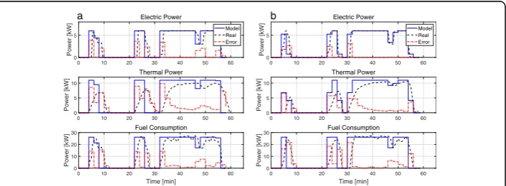
1. Calculation of the optimal load curves for one hour of operation using the presented mathematical model (See Fig.2)➔Pavailable
2. Transfer of the calculated set points to the combined heat and power plant➔Pset
3. Operation of the cogeneration plant for one hour to achieve the specified load profiles
4. Measurement of the actually achieved load profiles➔Preal
5. Repeating these steps by using the reference model [10] (See Fig.2).
Validation and results
the field test, the CHP is operated due to the set points given by the model. Nevertheless, the actual power output of the real CHP must be compared to the forecasted actual out-put of the mathematical model. In the reference model, the set point is equal to the fore-casted actual output. The results operated due to the optimization of both models are displayed in Fig.2. The forecasted actual power output and fuel consumption (“Model”) is compared to the actual output of the real CHP unit as a 30-s-average (“Real”) over the time horizon. The error is the mean deviation between“Model” and“Real”for each two minute time step. Both models show inaccuracies between the operational strategies given by the mathematical models and the real CHP unit. High inaccuracies occur especially during start-up processes. Nevertheless, the curves suggest that the model presented in this paper provides better operational strategies and output forecasts than the reference model, due to the extension of the power gradients constraints. Moreover, the time delay of the thermal power in the presented model reduces the error in the thermal power curve. Comparing both models by mean deviation errors, the presented model performs significantly better than the reference model (Fig.3). Overall, the evaluation of the field test shows that both mathematical models can only approximately represent reality. The presented model shows a significant improvement in comparison to the reference model, but further works must be done.
Table 2Technical data of the cogeneration unit.
Technical Parameter of the CHP Measurement technology used and its accuracy
Electrical power (Pmin) 3,0 kW Type DCMi 461 WP (Berg) +/, 3,5%
Electrical power (Pmax) 6,0 kWa
Electrical efficiency at maximum power (:ηelec,max)
23,4%a Calculated: (Electrical Power / Fuel Consumption)
+/−5%
Total Efficiency (:ηtotal) 64,6%a Calculated: ((Electrical power + Thermal Power) / Fuel Consumption)
+/−15%
Thermal Power 10,5 kWa Pump Magna 3 25–40 (Grundfos) +/−10%
Fuel consumption 25,5 kWa Type Aerius (Diehl Metering) +/−1,5%
a
Values are mean values measured in 5 h of operation
0 10 20 30 40 50 60
0 5 Power [kW] Electric Power Model Real Error
0 10 20 30 40 50 60
0 5 10
Power [kW]
Thermal Power
0 10 20 30 40 50 60
Time [min] 0 10 20 30 Power [kW] Fuel Consumption
0 10 20 30 40 50 60
0 5 Power [kW] Electric Power a b Model Real Error
0 10 20 30 40 50 60
0 5 10
Power [kW]
Thermal Power
0 10 20 30 40 50 60
Time [min] 0 10 20 30 Power [kW] Fuel Consumption
Conclusion
In this work, a mathematical modelling approach for CHP units was presented consid-ering real operating behaviours of CHP units in combination with a heat storage. The differentiation between set points and forecasted outputs in combination with a time delay in the thermal power output enable the better modelling of realty. Thus, the rela-tive error of the thermal output could be reduced in a field test with a real CHP unit from over 50% to 22% compared to the reference model. The error left is caused pri-marily by suboptimal parameterization. Moreover, power gradient constraints were tightened to a better fitting of real behaviour. Nevertheless, further researches require methods for more precise parameterization of the model via measurement data.
Abbreviations
CHP:combined heat and power plant; MILP: mixed integer linear programming
Acknowledgements
The authors gratefully acknowledge the financial support of the Kopernikus-Project“SynErgie”by the Federal Ministry of Education and Research (BMBF) and the project supervision by the project management organization Projektträger Jülich (PtJ).
Funding
Publication costs for this article were sponsored by the Smart Energy Showcases - Digital Agenda for the Energy Transition (SINTEG) programme.
Availability of data and materials
The datasets generated during and/or analysed during the current study are available from the corresponding author on reasonable request.
About this supplement
This article has been published as part ofEnergy InformaticsVolume 1 Supplement 1, 2018: Proceedings of the 7th DACH+ Conference on Energy Informatics. The full contents of the supplement are available online athttps:// energyinformatics.springeropen.com/articles/supplements/volume-1-supplement-1.
Authors’contributions
TW with the support of the remaining authors conceived of the presented idea. TW developed the modelling approach and JW supported the implementation of the model. NS and TK verified the analytical methods. Both carried out the field test and validation under notes and suggestions of TW. All authors discussed the results and contributed to the final manuscript. EA supervised the work. All authors read and approved the final manuscript.
Competing interests
The authors declare that they have no competing interests.
Publisher’s Note
Springer Nature remains neutral with regard to jurisdictional claims in published maps and institutional affiliations.
Published: 10 October 2018
References
Arroyo JM, Conejo AJ (2000) Optimal response of a thermal unit to an electricity spot market. IEEE Trans Power Syst 15(3): 1098–1104
Boji_C, M., Stojanovi_C, B.: MILP optimization of a CHP energy System (1996) Bosman, M.G.C.: Planning in smart grids. PhD thesis, S.l. (2012)
Bosman, M.G.C., Bakker, V., Molderink, A., Hurink, J.L., Smit, G.J.M.: On the microCHP scheduling problem (2009) Electric energy Thermal energy Fuel consumption
0 20 40 60
Mean deviation
error [%]
Presented model Reference model
Carrion M, Arroyo JM (2006) A computationally efficient mixed-integer linear formulation for the thermal unit commitment problem. IEEE Trans Power Syst 21(3):1371–1378
Christidis A, Koch C, Pottel L, Tsatsaronis G (2012) The contribution of heat storage to the profitable operation of combined heat and power plants in liberalized electricity markets. Energy 41:75–82
Costa A, Fichera A (2014) A mixed-integer linear programming (MILP) model for the evaluation of CHP system in the context of hospital structures. Appl Therm Eng 71:921–929
Fubara TC, Cecelja F, Yang A (2014) Modelling and selection of micro-CHP systems for domestic energy supply: the dimension of network-wide primary energy consumption. Appl Energy 114:327–334
Goldthau A (2014) Rethinking the governance of energy infrastructure: scale, decentralization and polycentrism. Energy Research & Social Science 1:134–140
Mitra S, Sun L, Grossmann IE (2013) Optimal scheduling of industrial combined heat and power plants under time-sensitive electricity prices. Energy 54:194–211
Poler R, Mula J, Diaz-Madronero M (2014) Operations research problems: statements and solutions. Springer, London Silvente J, Papageorgiou LG (2017) An MILP formulation for the optimal management of microgrids with task interruptions.
Appl Energy 206:1131–1146
Spieker, S.: Einsatz von BHKW mit Wärmespeicher im virtuellen Regelenergiekraftwerk (2013)
Steck, M.H.E.: Entwicklung und Bewertung von Algorithmen zur Einsatzplanerstellung virtueller Kraftwerke (2012) Steen D, Stadler M, Cardoso G, Groissböck M, DeForest N, Marnay C (2015) Modeling of thermal storage systems in MILP
distributed energy resource models. Appl Energy 137:782–792
Strasser T, Andren F, Kathan J, Cecati C, Buccella C, Siano P, Leitao P, Zhabelova G, Vyatkin V, Vrba P, Marik V (2015) A review of architectures and concepts for intelligence in future electric energy systems. IEEE Trans Ind Electron 62(4):2424–2438 Wang H, Yin W, Abdollahi E, Lahdelma R, Jiao W (2015) Modelling and optimization of CHP based district heating system