Cloud-Based Code Execution Framework for scientific problem solving environments

(1)

R E S E A R C H

Open Access

Cloud-Based Code Execution Framework for

scientific problem solving environments

Thomas Ludescher

1*

, Thomas Feilhauer

1

and Peter Brezany

2

Abstract

In this paper we present a novel Code Execution Framework that can execute code of different problem solving environments (PSE), such as MATLAB, R and Octave, in parallel. In many e-Science domains different specialists are working together and need to share data or even execute calculations using programs created by other persons. Each specialist may use a different problem solving environment and therefore the collaboration can become quite difficult. Our framework supports different cloud platforms, such as Amazon Elastic Compute Cloud (EC2) and Eucalyptus. Therefore it is possible to use hybrid cloud infrastructures, e.g. a private cloud based on Eucalyptus for general base-level computations using the available local resources and additionally a public Amazon EC2 for peaks and time-dependent calculations. Our approach is to provide a secure platform that supports multiple problem solving environments, execute code in parallel with different parameter sets using multiple cores or machines in a cloud environment, and support researchers in executing code, even if the required problem solving environment is not installed locally. Additionally, existing parallel resources can easily be utilized for ongoing scientific calculations. The framework has been validated by and used in our real project addressing large-scale breath analysis research. Its research-prototype version is available as a PaaS cloud service model. In the future researchers will be able to install this framework on their own cloud infrastructures.

Introduction

The project we are working on is driven by the breath research domain [1,2] but can be used for sim-ilar structured research area as well. In many scien-tific domains several different specialists (e.g. physician, mathematicians, chemists, computer scientists, etc.) are working together and executing long running CPU-intensive computations.

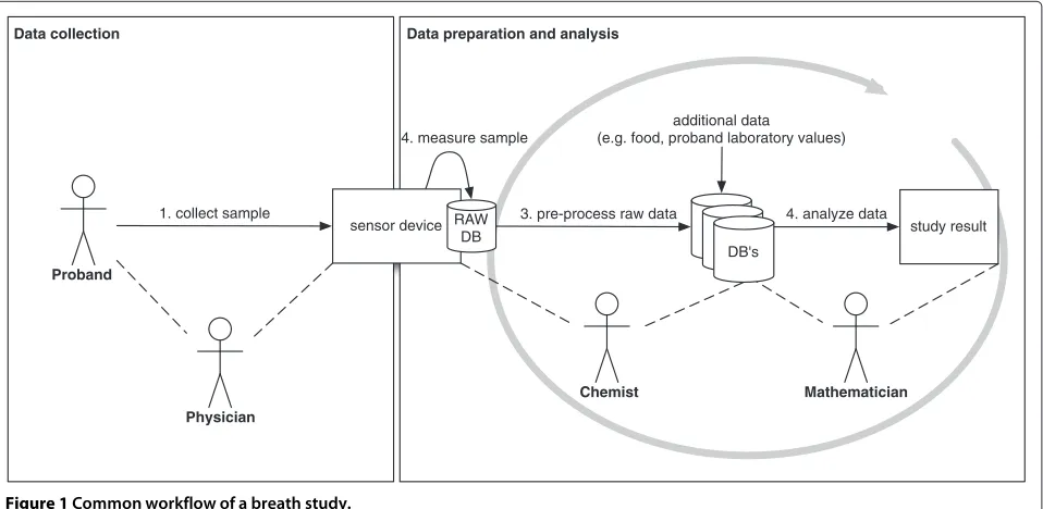
Figure 1 shows the common workflow of a scientific study with probands. Proband is a term used most often in medical fields to denote a particular subject (person or animal) being studied or reported on. Several different specialists, such as physician, medical researchers, tech-nician, chemists and mathematicians could be involved in a single study. In this example, sample data of a proband are collected and used for further analysis (e.g. breath

*Correspondence: [email protected]

1Fachhochschule Vorarlberg, University of Applied Sciences, Hochschulstrasse 1, 6850 Dornbirn, Austria

Full list of author information is available at the end of the article

sample, electrocardiogram data). At step (1), a physi-cian takes the sample of a proband and collects addi-tional information (e.g. smoker/non smoker). At step (2), the chemist measures the sample with several different sensors; each sensor device type generates its own raw data format. The chemist mostly uses a problem-solving environment, such as MATLAB, to pre-process the raw data (3). The mathematician uses the pre-processed data to create/adapt/improve/maintain new mathemati-cal algorithms (4). Depending on the goal of the study, different mathematical algorithms are performed (e.g. classification, pattern recognition, clustering, generate mathematical models). The mathematician must be able to recalculate the pre-processed data if required, even if the specific PSE is not installed locally. In our test example his/her results are the output of one single study.

The proposed Code Execution Framework (CEF) will support scientists to work together on the same study during all data preparation and data analysis steps, which could be executed recursively.

The following list outlines some challenges that we handle within this effort.

(2)

study result DB's

additional data

(e.g. food, proband laboratory values)

1. collect sample

Physician

Chemist Mathematician

Proband

DB's DB's

Data collection Data preparation and analysis

sensor device RAW DB

3. pre-process raw data 4. analyze data 4. measure sample

Figure 1Common workflow of a breath study.

• All involved specialists will iteratively improve this workflow during the development phase. To increase these iterative steps, each researcher should be able to use his/her favorite problem solving environment. At the moment MATLAB [3], Octave [4] and R [5] are supported. The CEF has been implemented in an ongoing project with the breath analysis community. In this domain the researcher mostly uses MATLAB for pre-processing the data and R or MATLAB for all further mathematical analysis.

• Different specialists use different PSEs for their calculations and provide their results to other scientists for further analysis, probably with another PSE. For example a chemist uses MATLAB to prepare the input data of a mass-spectrometry to identify the required substances and a statistician uses this data to generate statistical analysis in R. That means that two different PSEs must work together within a single study.

• Each scientist must be able to execute different problem solving environment source files out of his/her favorite PSE, without having the other PSE installed. This is especially important for non open source or free PSEs, such as MATLAB. The CEF provides a solution to execute MATLAB code without having MATLAB installed.

• Long running calculations block the computer of the scientists and in terms of a failure (e.g. no disk space) the whole calculation may fail. If the scientist uses the CEF it will manage the failure recovery and invoke the calculation at a new machine again. Additionally, the client computer is free for

other uses.

• Nowadays most desktop computers have multiple cores or even multiple processors. MATLAB already supports multi-threaded computation for a number of functions [6]. Some problem solving environments (e.g. Octave and R) are generally single-thread applications. However, these PSEs use existing numeric libraries that can take advantage of parallel execution. R and Octave provide different toolboxes to support multiple cores or the scientist must start the PSE several times for different calculations. Within the CEF, the user specifies the specific method that should be executed in the cloud with different parameter sets in parallel. The results will be merged together and returned back to the

client.

The goal of the proposed CEF is to support multi-ple different problem solving environments and to exe-cute long running CPU-intensive calculations in parallel in a cloud infrastructure. Depending on the require-ments of the user, specific calculations must be fin-ished within a certain amount of time. The system can be configured to use a local Eucalyptus instal-lation meeting the demand for base level computa-tions; if required, Amazon EC2 instances can be con-nected to speed up (bursting) the calculations (hybrid cloud). This can have advantages in terms of time and costs.

(3)

even if the required problem solving environment is not installed locally, (c) allowing the CEF-clients to use the research prototype as a Platform as a Service (PaaS) solu-tion, and (d) in the future, the whole CEF will be offered for a local installation using an own cloud platform.

The rest of the paper is organized as follows. Section ‘Background and related work’ gives some background information about problem solving envi-ronments, parallel execution services, cloud environ-ments, and workflow management systems. The usage of the CEF can be seen in Section ‘Usage of the Code Execution Framework within different PSEs’. In Section ‘Code Exe- cution Framework (CEF) con-cept’ the CEF is specified and all involved compo-nents are defined. Section ‘Implementation’ describes the the prototype implementation. Section ‘Performance tests’ contains the performance results. At the end the open problems and our future work are described in Section ‘Open problems and future work’.

Background and related work

Cloud computing [7] provides computation, software, data access, and storage resources without requiring cloud users to know the location and other details of the computing infrastructure. In general, the amount of data is growing rapidly and the systems process-ing this data must deal with several data management challenges. Moshe Rappoport [8] outlines the chal-lenges as the four V’s: the Volume, Variety, Velocity and Veracity. This big amount of data must be analyzed with innovated technologies to discover new knowledge. The book [9] presents the most up-to-date opportu-nities and challenges emerging in knowledge discov-ery in big data, helping readers develop the technical skills to design and develop data-intensive methods and processes.

According to the applied deployment model, the cloud infrastructure can be divided into public clouds, com-munity clouds, private clouds, and hybrid clouds [10]. The difference between these groups are the location, owner, payment, and user. Several different cloud plat-forms exist, such as Amazon Web Service (AWS) [11], Eucalyptus [12], and so on. Each cloud infrastructure uses its own storage resources. At AWS it is called S3 [13], at Eucalyptus they use Walrus. Walrus is an open source implementation of S3 and provides the same interface. Different types of service models can be accessed on a cloud computing platform - the most favorite types include Infrastructure as a service (IaaS), Platform as a Service (PaaS) and Software as a Service (SaaS).

A Problem Solving Environment (PSE) is a specialized computer application for solving mathematical or statisti-cal problems, mostly with a graphistatisti-cal user interface [14].

Many scientific research groups use PSEs, such as MAT-LAB [3], Octave [4] and R [5] for their calculations. For example, in [15] several different applications of MATLAB in science and engineering are shown.

Considering parallel execution services, there are sev-eral frameworks described in the literature, such as ParallelR [16], NetWorkSpace for R [17], RevoDeployR [18], and Elastic-R [19] for executing R code in paral-lel. There are packages and extensions for MATLAB and Octave including Parallel-Octave [20], Multicore [21], and MatlabMPI [22].

There exists already some Web/cloud based tools to remotely communicate with PSEs. There are two differ-ent approaches to use MATLAB within the Cloud. The first approach was developed by MathWorks and uses concrete licenses (e.g. MATLAB Distributed Comput-ing Server license). The latter one uses the Component Runtime (MCR) of MATLAB, which does not require licenses for each node. The white paper [23] describes the MathWorks approach in detail. This white paper walks you through the steps of installation, configuration, and setting up clustered environments using these licensed products from MathWorks on Amazon EC2. This license based approach is very expensive, depending on the num-ber of nodes. The advantage of using the Parallel Toolbox is to be able to execute even a for-loop in parallel on different nodes. It is possible to use Red Cloud [24] as a Cloud Service (IaaS) to execute MATLAB code with the MATLAB Distributed Computing Server. With the MCR-approach it is possible to develop a WebService without any costs for licenses. In the paper [25] exactly this approach was addressed within the Grid infrastruc-ture. As further work, the author mentioned that they would like to find out how GridMate behaves on Cloud resources.

With Octave and R, which are developed under the GNU license, all license problems are solved. There already exists a possibility to use Octave as a Cloud Ser-vice [26]. With the R-Cloud workbench [27] it is possible to execute R code in parallel in a provided cloud infras-tructure (R-Cloud). For R there are solutions to execute R in the Amazon EC2 Cloud [28].

(4)

in a heterogeneous environment, as well. For exam-ple, it is possible to execute R code within an Octave code execution.

Workflow engines, such as Taverna [30], Kepler [31], ClowdFlows [32], and ADAMS [33], can be used to orchestrate analysis tasks in a workflow. A user of a workflow management system is able to define its own workflows and execute it. A workflow can consist of data services, calculation services, and other services. Our system does not directly include any workflow engine. However, with our CEF it is possible to execute arbitrary R/Octave and MATLAB code in the cloud. The frame-work provides a Web service interface that can be used within a complex workflow to execute PSE code in paral-lel. We have already implemented a Taverna activity that is based on these CEF Web services.

In many domains, personal data (e.g. patient data) is involved and therefore privacy and security are very important. The proposed CEF uses a Kerberos based security concept. In [34] we discussed several challenges and their solution, including how to (a) use client authen-tication through all levels of the system, (b) guarantee secured execution of time consuming cloud based anal-ysis, and (c) inject security credentials into dynamically created virtual machine instances.

Usage of the Code Execution Framework within different PSEs

In this section, we will demonstrate how the CEF can be used to execute MATLAB or R code in parallel in the cloud. The corresponding Octave code can be implemented in a similar way. To illustrate the usage of the framework, we calculate PI with a Monte-Carlo method [35] as an example for a compute intensive job that can easily be parallelized. This example will be used in Section ‘Performance tests’ for the performance evaluation.

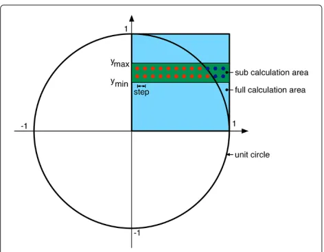
To execute the Monte-Carlo method in parallel, we put a grid over the unit circle (Figure 2) and calculate the num-ber of points in the circle and the total numnum-ber. PI can be calculated with the following formula

=4·

number_of_points_in_circle

total_number

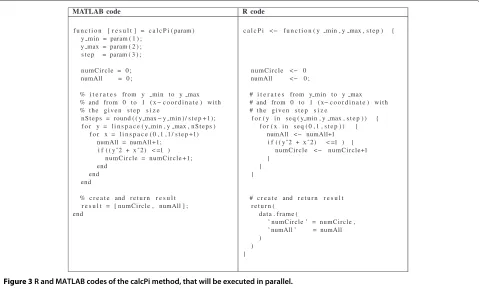
First of all the provided MATLAB or R Code Execution Library must be installed. Secondly we must implement the MATLAB function that should be executed in paral-lel, as described above. This function uses one array as parameter with 3 values. The first value contains ymin, the second value ymax, and the last value is the step size. The code iterates from ymin to ymax and from 0 to 1 (x-coordinate) with the given step size and calculates the number of values inside the unit circle (numCircle) and the total number (numAll).

Figure 2Area selection of the unit circle.

Theyminandymaxparameters are used to select a spe-cific area of the unit circle. Figure 3 shows the calcPi code that calculates the numbers of points inside the unit circle (numCircle) and the total number (numAll).

Figure 4 shows the codes (MATLAB and R) to (a) gener-ate the parameter sets, (b) make a connection to the Code Execution Controller (CEC), (c) execute the calcPi func-tion, and (d) load the calculated result from the CEC. With the three parameters of the CodeExecution constructor you are able to specify whether you would like to execute the calculation in the cloud or locally (1st parameter), the domain name and the port of the used CEC, and whether you would like to use the GUI login or the console login. During the development phase the scientist is able to test her/his method at her/his local machine (the required PSE must be installed). By adopting the first parameter, the whole code will be executed at the cloud based Code Execution Infrastructure.

At the executeCalculation method the scientist must provide the different parameter sets, the method name that should be executed in parallel, and whether this method should be blocked (synchronous) until the parallel execution in the cloud is finished.

(5)

MATLAB code R code

f u n c t i o n [ r e s u l t ] = c a l c P i ( param ) y min = param ( 1 ) ;

y max = param ( 2 ) ; s t e p = param ( 3 ) ; n u m C i r c l e = 0 ; numAll = 0 ;

% i t e r a t e s from y min t o y max % and from 0 t o 1 ( x − c o o r d i n a t e ) w i t h % t h e g i v e n s t e p s i z e

n S t e p s = round ( ( y max − y min ) / s t e p + 1 ) ; f o r y = l i n s p a c e ( y min , y max , n S t e p s )

f o r x = l i n s p a c e ( 0 , 1 , 1 / s t e p +1) numAll = numAll +1;

i f ( ( y ˆ2 + x ˆ 2 ) < =1 ) n u m C i r c l e = n u m C i r c l e +1; end

end end

% c r e a t e and r e t u r n r e s u l t r e s u l t = [ numCircle , numAll ] ; end

c a l c P i <− f u n c t i o n ( y min , y max , s t e p ) {

n u m C i r c l e < − 0 numAll <− 0 ;

# i t e r a t e s from y min t o y max # and from 0 t o 1 ( x− c o o r d i n a t e ) w i t h # t h e g i v e n s t e p s i z e

f o r ( y i n s e q ( y min , y max , s t e p ) ) { f o r ( x i n s e q ( 0 , 1 , s t e p ) ) {

numAll <− numAll+1 i f ( ( y ˆ2 + x ˆ 2 ) < =1 ) {

n u m C i r c l e < − n u m C i r c l e+1 }

} }

# c r e a t e and r e t u r n r e s u l t r e t u r n (

d a t a . fr a m e (

’ numCircle ’ = numCircle , ’ numAll ’ = numAll )

) }

Figure 3R and MATLAB codes of the calcPi method, that will be executed in parallel.

% max num o f sub − c a l c u l a t i o n s numCalc = 20

% s t e p width s t e p = 0 . 0 0 0 0 5 ;

% c r e a t e params ( f i r s t q u a d r a n t ) tmp = l i n s p a c e ( 0 , 1 , numCalc + 1 ) ; params = [ ] ;

f o r num = 1 : numCalc params (num , : ) = [

tmp (num)+ s t e p , tmp (num+1) , tmp ] ; end

params ( 1 , 1 ) = 0 ;

% i n i t i a l i z e Code E x e c u t i o n C o n t r o l l e r c e = CodeExecution (

t r u e , % u s e CEF

’DNS :PORT’ % URL o f C o n t r o l l e r t r u e % u s e l o g i n GUI ) ;

% e x e c u t e c a l c u l a t i o n c a l c = c e . e x e c u t e C a l c u l a t i o n (

params , % p a r a m e t e r s ’ c a l c P i ’ , % method name t r u e % b l o c k c a l c u l a t i o n ) ;

% l o a d r e s u l t s

r e s u l t s = c e . g e t C a l c u l a t i o n R e s u l t s ( c a l c ) ;

# max num o f sub − c a l c u l a t i o n s numCalc <− 20

# s t e p width s t e p <− 0 . 0 0 0 0 5

#c r e a t e param ( f i r s t q u a d r a n t ) tmpArray <− s e q ( 0 , 1 , 1 / numCalc ) params <− r b i n d ( )

f o r (num i n 1 : numCalc ) { params <− r b i n d ( params ,

c ( tmpArray [ num]+ s t e p , tmpArray [ num+ 1 ] , s t e p )

) }

params [ 1 , 1 ] <− 0

# i n i t i a l i z e Code E x e c u t i o n C o n t r o l l e r c e <− i n i t C o d e E x e c u t i o n (

TRUE, # u s e CEF

DNS :PORT” # URL o f C o n t r o l l e r TRUE # u s e l o g i n GUI )

# e x e c u t e c a l c u l a t i o n c a l c <− e x e c u t e C a l c u l a t i o n (

ce , # CE c o n n e c t i o n params , # p a r a m e t e r s

’ c a l c P i ’ , # method name TRUE # b l o c k c a l c u l a t i o n )

# l o a d r e s u l t s

r e s u l t <− g e t C a l c u l a t i o n R e s u l t s ( ce , c a l c )

(6)

% i n i t i a l i z e Code E x e c u t i o n C o n t r o l l e r c e = CodeExecution (TRUE, ’DNS :PORT’ ) ; % download e x i s t i n g PSE c o d e

c e . l o a d C a l c u l a t i o n C o d e (

1 2 3 4 , % c a l c u l a t i o n ID ’ c o d e . z i p ’ % o u t p u t f i l e n a m e )

% i n i t params , a s a l r e a d y shown . . .

% e x e c u t e c a l c u l a t i o n w i t h z i p f i l e c a l c = c e . e x e c u t e C a l c u l a t i o n F r o m Z i p ( params , % p a r a m e t e r s ’ c o d e . z i p ’ , % i n p u t f i l e n a m e t r u e % b l o c k c a l c u l a t i o n )

% l o a d r e s u l t s , a s a l r e a d y shown . . .

# i n i t i a l i z e Code E x e c u t i o n C o n t r o l l e r c e <− i n i t C o d e E x e c u t i o n (TRUE, ”DNS :PORT” ) # download e x i s t i n g PSE c o d e

l o a d C a l c u l a t i o n C o d e ( ce , # CE c o n n e c t i o n 1 2 3 4 , # c a l c u l a t i o n ID ’ c o d e . z i p ’ # o u t p u t f i l e n a m e )

# i n i t params , a s a l r e a d y shown . . .

# e x e c u t e c a l c u l a t i o n w i t h z i p f i l e c a l c <− e x e c u t e C a l c u l a t i o n F r o m Z i p (

ce , # CE c o n n e c t i o n params , # p a r a m e t e r s ’ c o d e . z i p ’ , # i n p u t f i l e n a m e TRUE # b l o c k c a l c u l a t i o n )

# l o a d r e s u l t s , a s a l r e a d y shown . . .

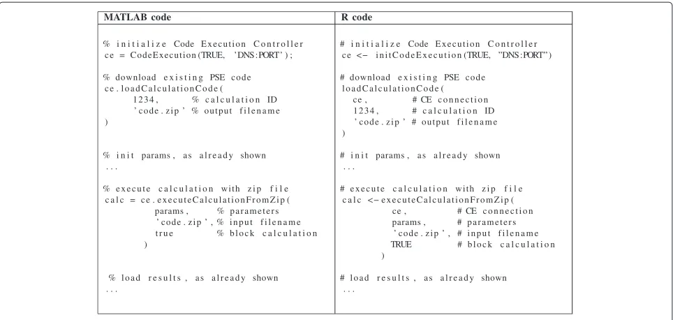
Figure 5R and MATLAB codes to download already executed calculations and recalculate it.

Execution Framework (CEF) concept’), can be used in the same way asexecuteCalculationorgetCalculationResults.

Code Execution Framework (CEF) concept

In the following sections, the concept of the CEF will be described. We start with describing how the CEF access activation is selected by the specific system parameter useCEF accepting the values FALSE and TRUE. If the value useCEF is FALSE, the whole calculation will be executed in the PSE on the local machine separately. The scientist is able to use all features of the PSE, such as debugging, printing, but must wait until the calcula-tion is completely finished. Without parallel extensions a PSE uses only one core. Depending on the power of the computer used, long running calculations can take a while. If the scientist setsuseCEFto TRUE, the CEF will be used. The Code Execution Controller starts the required amount of VMs, transmits the calculation to VMs, exe-cutes the calculations, and generates the combined result. The administrator of the CEF must define which cloud platforms (e.g. Amazon EC2, Eucalyptus) are used. For each cloud platform he/she must set (a) what machines types should be used (e.g. m1.small, m1.xlarge), (b) how many instances can be started simultaneously, (c) the shut down behavior (e.g. shut down immediately after all waiting calculations are finished or just before the researcher has to pay for another hour for this idle machine), and (d) the total available daily/monthly budget for this cloud platform. The Code Execution Controller (CEC) is able to call the WorkerNodeStatus Web ser-vice from each VM to request the number of available cores, core usage, total and available memory. At the

moment the CEC starts the maximum available amount of virtual machines if required, the maximum cost bound-ary is not yet implemented. The CEC stores all started VMs in a queue. If a calculation is waiting, the first free VM will be used for this execution. In terms of security, the worker node (VM) only accepts requests of the CEC that started the VM. When the calculation at a worker node is finished or failed, the result and log information will be sent to the CEC and afterwards all files from this calculation will be deleted immediately. In the future, the CEC will send sub-calculations from one user to a worker node at the same time, even if multiple cores are available. Therefore it is impossible to spy out data of other users by executing dangerous PSE code.

The advantages for the scientists are (a) the result will be available much faster than running locally, (b) the sci-entists can use the client computer for other purposes, (c) the scientist can look up the status of the calculation at the CEF-Portal, (d) the scientist is able to download the result to another computer, and (e) the scientist is able to execute other PSE code, even if the required PSE is not installed locally.

(7)

Figure 6Code Execution Framework overview.

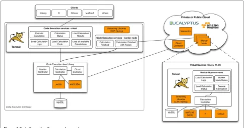
Components description

In the section we describe the components in detail.

Code Execution Controller (CEC)

The CEC consists of the Code Execution Java Library, two different Web service groups (client and worker node services), and a MySQL database to store all calculations and sub-calculations. The Java library is at the heart of the CEF. It provides methods to produce sub-calculations, start and stop virtual machines, to copy the code to be executed into S3 (AWS) or Walrus (Eucalyptus), as well as to monitor running calculations and virtual machines. The CEF supports parallel code execution on the level of executing methods in parallel with different parameter sets.

The client Web services support online execution of functions, methods, and scripts written in different PSEs (e.g. MATLAB, R, Octave, etc.). The user of the system communicates with the client Web services while worker node services are used only internally. In the following these two groups of services are described.

• Client services - These services must be invoked by one of the clients (e.g. Octave, MATLAB, R, Liferay and Taverna). They include

– Execute Calculation - this service can be used to start a new calculation. In order to execute a new calculation, all parameters for

parallelization needed in the code are passed

as comma-separated values to the service. At the beginning, this service generates parallel executable sub-calculations (same method with different parameters). Afterwards the PSE code will be stored at S3/Walrus to reduce time and data transfer for parallel execution. Finally, the sub-calculations will be transmitted to a free worker node virtual machine (VM) to be executed.

– Calculation Status - this service allows for the monitoring of the code execution by

requesting the current status, which can either becompiling, waiting, running, finished, or error. The status can be requested either for the entire calculation or for each sub-calculation.

– Load Calculation Results - this service loads the results from either the entire calculation or from each sub-calculation.

– Load Calculation Logs - this service loads the logs from sub-calculations. This includes all output on the console from the used PSE. – Load Calculation Code - this service can be

(8)

the execution with the same parameter set will be faster than without the compiled code. The CEC recognizes the compiled code and skips the compilation step, depending on the amount of code this can last from some seconds up to a couple of minutes.

– Load All Available Calculations - this service returns all accessible calculations of the authenticated user. The Code Execution Liferay [37] portlet uses this method to show an overview on the calculations.

• Worker Node services - These services will be invoked by the worker node VM. They include

– Calculation Finished - this service informs about successfully finished sub-calculations and receives the calculation results and logs from the VM.

– Calculation Finished with Failure - in case the calculation finished with errors, then this service receives the calculation logs from the VM.

Supported clients

The CEF will be easily accessible from different clients. Each user is able to communicate with the CEF from within R/Octave/MATLAB, the workflow engine Tav-erna, or even from the Web without needing to install any specific environment. To support Taverna we imple-mented a Taverna activity, that is able to use the Web services of the CEF. We provide several differ-ent R/Octave/Matlab code examples (e.g. PI calculation, recursive CEF invocation, download code and re-execute the downloaded code). All Web services described above can be used with these client libraries, and have been tested on Windows, Linux, and OS X. Additionally, a researcher is able to start new calculations or monitor running calculations within our Web portal (Liferay). Each client/toolbox communicates with the client CEC Web services.

Cloud infrastructure

The CEF uses the EC2 API to communicate with the cloud infrastructure. The controller needs to start/stop instances on the cloud and store data within the data stor-age (Walrus/S3). All these steps can be done with the AWS SDK for Java and the Jets3t library.

Code Execution Framework virtual machine

We provide a specific worker node virtual machine (Ama-zon EC2 and Eucalyptus) for the execution of the different PSE code. On this VM all three PSEs (R, Octave, MATLAB

Component Runtime) are installed and a Tomcat applica-tion server is running, hosting Code Execuapplica-tion Services of the CEF.

The worker node Web application provides several dif-ferent Web services for the CEC. They include:

• Execute Calculation - this service can be used to start a new calculation at the specific worker node. In order to execute a new calculation all parameters needed in the code are passed as comma-separated values to the service. The worker node downloads the required PSE code from the Walrus/S3. All

information or error outputs will be stored in files during the whole calculation. After the calculation is finished or failed the result and log information will be sent back to the CEC and all files will be deleted. • Worker Node status - this service returns

information about the worker node, such as total and used memory, number of available cores, used cores, etc. The worker node uses the SIGAR (System Information Gatherer And Reporter) Java library to request the required values from the machine. • Load Calculation status - this service returns

information about one specific sub-calculation, such as used memory, used CPU, etc.

• Load Calculation Logs - this service returns the log of a running calculation.

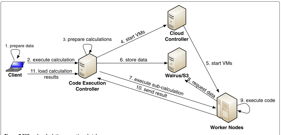
Execution sketches

In this section we walk through a complete execution sketch.

(9)

Code Execution Controller

Walrus/S3 Cloud Controller

Worker Nodes Client

2. execute calculation

3. prepare calculations

4. start VMs

5. start VMs 6. store data

7. execute sub-calculation 8. request data

9. execute code 10. send result

1. prepare data

11. load calculation results

Figure 7PSE-code calculation execution sketch.

the data preparation the client invokes the executeCal-culation Web service at the CEC (step 2). The Code Execution Controller (a) stores the received data on the disk, (b) compiles the MATLAB source code, if required (for further information have a look at Section ‘MAT-LAB Component Runtime approach’), (c) generates the sub-calculations, (d) adds all sub-calculations to the cal-culation queue (step 3), and (e) starts additional Code Execution VMs, if required (step 4, step 5). A specific thread processes the calculation queue. For each calcu-lation the code will be sent once to the Walrus or S3, depending on the cloud infrastructure used (step 6). This reduces the amount of transmitted data and the required time and costs. Afterwards the sub-calculation will be executed at an idle Code Execution VM(step 7). The worker node (a) requests the Code from Walrus/S3 (step 8), (b) executes the code in the shell (step 9), (c) generates the result CSV, (d) sends the result back to the CEC (step 10), and (e) deletes all generated files. Step (e) is important to keep a minimal amount of free disk space, otherwise we have to start a new instance if the Worker Node has not enough free disk space for further calculations. Additionally this must be done because of security reasons. At the end of the execution, the CEC checks the received data and updates the status informa-tion of the calculainforma-tion. The researcher is able to request the status of the calculation (e.g., running, finished) and the results. Therefore the client invokes the loadCalcula-tionResult Web service method with the id to download the result (step 11). The CEC (a) authorizes the user, (b) checks if the calculation is finished, and (c) gener-ates the result CSV. At the end, the client converts the

received CSV result set to the internal data structure of the corresponding PSE.

MATLAB Component Runtime approach

(10)

At our online test installation no additional toolboxes are installed. With this step, every user of the CEF is able to execute MATLAB source files without having to buy a MATLAB license.

MathWorks products license example

To calculate the license cost with and without CEF, the following six assumptions are made: (1) the com-pany is allowed to use the academic price list (2013); (2) five researchers of the company are using Matlab at their computers (individual licenses); (3) all researchers must have all six Computational Finance toolboxes (financial toolbox, econometrics toolbox, datafeed tool-box, database tooltool-box, spreadsheet Link EX, and finan-cial instruments toolbox); (4) the license for MATLAB itself costs e500 (single named user or single com-puter); (5) all Computational Finance toolboxes cost e200 each; (6) the MATLAB Compiler toolbox costse 500.

With these assumptions without CEF the total license costs aree8500 (for each user the MATLAB license costs and additionally all six Computational Finance toolboxes). In the best case with CEF the total license costs aree2200 (one MATLAB license costs for a single machine, all six Computational Finance toolboxes, and additionally the MATLAB Compiler toolbox). You must take into account, that without having a valid MATLAB license for each user the development process is more complicating (e.g. no debugging, no GUI, no auto completion).

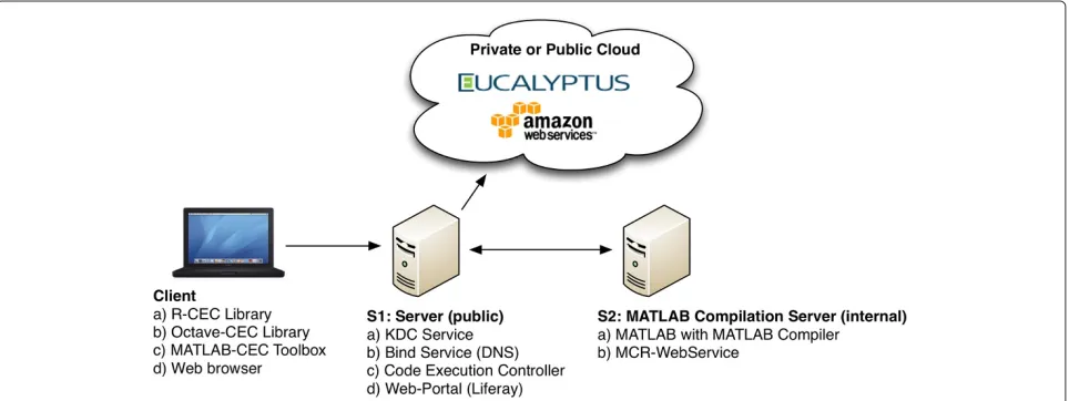
Implementation

In this section, detailed information about the implemen-tation is given. Each component provides different Web services as described in Section ‘Code Execution Frame-work (CEF) concept’. All Web services are implemented

with CXF [40]. The data (PSE source code and CSV parameters) are streamed with MTOM [41]. In our project personal related data is involved and we must implement a fitting security concept. The whole CEF is implemented with a Kerberos based security concept which has been described earlier by us in [34].

Figure 8 gives an overview on our prototype. The figure depicts all involved components. Server 1 (S1, Ubuntu 11.04) is connected to the Internet with a public IP address, located at the university of applied sciences in Dornbirn; this is necessary to be able to use the system outside of the private institute network. This machine is used for several different services. The Key Distribu-tion Center (KDC) and the DNS-Service are used for our Kerberos based security framework. The CEC manages and monitors all calculations. The Web-Portal (Liferay) can be used to monitor calculations without having any PSE installed. Server 2 (S2, Ubuntu 11.04) has a MAT-LAB with the Compiler toolbox installed. Additionally the own-implemented Web Service to compile MAT-LAB code is running in the Tomcat on this machine. As Cloud infrastructure, we tested our own Eucalyptus (2.0) and Amazon EC2. Theoretically, all other EC2 compat-ible cloud infrastructures should work with our system, however we have not tested it so far. Most likely, the VM image must be created for each cloud infrastruc-ture separately. There exist discrepancies how the assign-ment of internal IP addresses of the VM must be done. At the moment, we provide an image for Amazon EC2 and Eucalyptus. All different cloud infrastructures can be combined to a hybrid system. This can have advan-tages in terms of speed and costs. The Code Execution Framework can be used in several different ways. The sci-entist at the client side has to use one of the provided interfaces.

(11)

The VM (Ubuntu 11.04) that is used to execute jobs from the CEC contains:

• Startup Tool - This tool will be executed after booting the VM. It (a) requests the required security information from the CEC, (b) downloads a zip file from the storage controller that contains additional files and scripts, (c) downloads the Web application for the Worker Node from the storage control, and (d) starts the Web application within the Tomcat (7.0) application server. Step (b) is used to be able to change the VM (e.g., install libraries, execute shell scripts, etc.) without creating a new VM. We use this feature during our framework development phase. • Worker Node Web Services - This Web application

only accepts requests from the corresponding CEC and manages and monitors all running calculations. • PSEs - To be able to execute R and Octave code,

these libraries with all required toolboxes must be installed. To execute compiled MATLAB code, the VM needs to have the MATLAB Compiler Runtime (MCR) installed.

At the moment, it is possible to test the CEF with your Web portal [36], the R-Client. You are allowed to use our test CEF infrastructure with two worker nodes to execute R, Octave, or already compiled MATLAB code. For more information have a look to the Online-Demo page at our Web portal.

Performance tests

The Code Execution VM is provided for both, AWS and Eucalyptus Cloud platforms. The key performance characteristics are compute, memory, I/O bound. At the moment, the breath analysis community uses mostly CPU intensive calculations and we decided to eval-uate the overhead for these criteria. Therefore most relevant performance measures for our application are number of CPUs, size of memory, and data transfer rates (while using a hybrid infrastructure). Therefore we have defined performance evaluations based on these criteria.

The results of the evaluation represent important infor-mation aiming to predict the overhead of different infras-tructures, which is required to generate the best possible execution plan if multiple cloud platforms are available. To predict the required execution time, we need to execute at least one sub-calculation.

During the following performance tests we found sev-eral important results:

• The execution time for our test calculation mainly depends on the cloud infrastructure used and the problem solving environment used.

• MATLAB is the fastest PSE for executing our time consuming PI calculation, even if we need to compile the PSE code.

• The boot procedure of a VM depends not only on the used virtual machine type: The VM must be

transmitted from the S3/Walrus to the host node, if it is not already in the cache.

• The transfer speed between CEC and VM cannot be neglected, especially if the internet connection is slower and large data sets must be

transmitted (e.g., input data, code, parameter).

In the following paragraphs we provide the detailed results of our performance tests.

In order to evaluate the first prototype of our Code Execution Services, we have conducted three different experiments. In the first experiment we tested the exe-cution time with CPU intensive MATLAB, Octave, and R examples in order to measure the VM overhead and the performance of the whole framework; in the second test we tried to retrieve the rate for the data transfer, and in the last experiment we measured the boot time of the Code Execution VM. A small Eucalyptus private cloud has been installed at our lab at the University of Applied Sciences.

We have implemented Monte-Carlo methods [35] cal-culating PI in MATLAB, R, and Octave as shown in Section ‘Usage of the Code Execution Framework within different PSEs’. This PI calculation is CPU intensive and can easily be parallelized. Calculating PI is one of the major cloud (MapReduce) evaluation use cases [42,43]. The calculations were executed in different code exe-cution scenarios: (a) local (1 thread), (b) on a private Eucalyptus cloud, (c) on Amazon Elastic Compute Cloud (EC2), and (d) on a hybrid cloud (Eucalyptus and Amazon Elastic Compute Cloud). All tests have been executed 50 times and the results are arranged in the following tables showing the arithmetic means and standard deviation of the measured values.

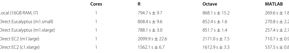
Evaluation of the VM overhead

(12)

Table 1 Evaluation of the VM overhead

Cores R Octave MATLAB

Local (16GB RAM, I7) 1 794.7 s±9.7 868.1 s±15.2 269.6 s±1.8

Direct Eucalyptus (m1.small) 1 808.4 s_±9.6 852.4 s_±1.6 270.8 s_±2.2

Direct Eucalyptus (m1.xlarge) 1 788.1 s±3.0 851.7 s±1.4 257.4 s±2.7

Direct EC2 (m1.large) 1 2099.9 s±22.6 2171.0 s±7.5 710.7 s±0.9

Direct EC2 (c1.xlarge) 1 1562.1 s±6.7 1612.9 s±3.3 537.5 s±0.8

The values are given as mean±standard deviation.

or Octave (868.1 s). This should be taken into account for choosing the appropriate PSE for a specific calculation.

The overhead of the local machine (i7) and the Euca-lyptus VM (m1.small) is minimal (for R about 1.5%, for MATLAB about 0.5%). Therefore the VM overhead can be ignored for our further performance analysis. It is interesting to see that the Amazon calculation (m1.large) takes up to 2.6 times longer than the Eucalyptus or even the local execution (compute intensive and non-memory bound). To verify this overhead we decided to use another CPU intensive test example as shown in [44]. For this test we used the commandtime for i in 0..10000; do for j in 0..1000; do :; done; donein the terminal. At the local machine, the execution takes 19 seconds, in EC2 with the m1.large 47 sec and with c1.xlarge 37 seconds. With this test, the EC2 (m1.large) takes about 2.5 times longer than the local execution, which means approximately the same performance overhead as with the CEF. In [45] Amazon describes EC2 compute units:“In order to make it easy for developers to directly compare CPU capacity between different instance types, we have defined an Amazon EC2 Compute Unit. The amount of CPU that is allocated to a particular instance is expressed in terms of these EC2 Compute Units. We use several benchmarks and tests to manage the consistency and predictability of the perfor-mance of an EC2 Compute Unit. One EC2 Compute Unit provides the equivalent CPU capacity of a 1.0–1.2 GHz 2007 Opteron or 2007 Xeon processor.”That is the reason why it is not possible to compare one EC2 instance with a local machine with a specific CPU.

Table 2 R performance evaluation

Cores Seconds Speed-up

3×Eucalyptus (m1.small) 3 301.1 s±3.2 2.64

2×Eucalyptus (m1.xlarge) 4 242.8 s±5.3 3.27

3×AWS (m1.large) 6 342.2 s±4.7 2.32

1×AWS (c1.xlarge) 8 285.3 s±4.6 2.79

and 1_×AWS (c1.xlarge)

Code Execution Framework performance analysis

Table 2 shows the R performance evaluation, Table 3 the Octave performance evaluation, and Table 4 the MAT-LAB performance evaluation. In the last column we show the speed-up of the CEF execution in comparison to the local usage. With R and Octave, the theoretically opti-mal values can almost be reached. With three Eucalyptus VMs (3x m1.small - 3 cores), the theoretical speed-up is 3, while our measured values are 2.64 (R) and 2.71 (Octave). The overhead of the CEF, including the nec-essary data transfer, is therefore approx. 10%. With two Eucalytpus VMs (2x m1.xlarge - 4 cores), the speed-up is 3.27 (R) and 3.37 (Octave). At Amazon Elastic Compute Cloud, the speed-up of the CEF execution in compari-son to the local usage is not able to reach the theoretical value (e.g. 2.32 instead of 6). You must take in account, that, for example, using R, the single execution in EC2 (m1.large: 2099.9 s) takes much longer than the local one (794.7 s).

The reasons why we could never reach exactly the theo-retically optimal value are (a) different CPU types in EC2 and AWS, (b) overhead for splitting calculations into sub-calculations, (c) overhead for distributing sub-calculations to free worker nodes, (d) overhead for converting the transmitted CSV-parameters to internal data structures of the used PSE, (e) data transfer time for the parameter and the code, and (f ) number of sub-calculations cannot be divided by the number of cores without there being a remainder of tasks. Issue (f ) is especially important for tests with several cores (e.g. 6, 8, or 12).

Table 3 Octave performance evaluation

3×AWS (m1.large) 6 449.7 s±6.5 1.93

1×AWS (c1.xlarge) 8 265.0 s±3.0 3.28

and 1_×AWS (c1.xlarge)

(13)

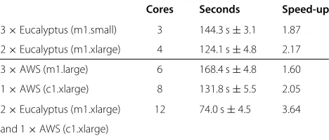
Table 4 MATLAB performance evaluation

3×AWS (m1.large) 6 168.4 s±4.8 1.60

1×AWS (c1.xlarge) 8 131.8 s±5.5 2.05

and 1×AWS (c1.xlarge)

Table 4 shows the measured results of the execution of the compiled MATLAB code. By increasing the number of cores, the calculation time is reduced, but the theoret-ical speed-up value cannot be reached (e.g. 1.87 instead of 3). The reason for this is that the worker node needs a certain amount of time to start the MATLAB Component Runtime Environment (MCR). To reduce the MCR over-head and the Web service, overover-head each sub-calculation should be a long running calculation. If a sub-calculation is completed fast enough, it is possible to send multiple sub-calculations within one Web service call.

The compilation of our test MATLAB code takes in average 39.1 seconds. This contains (a) the Web service invocation, (b) transfer of source code to the MATLAB compiler Web service, (c) compilation of the source code, and (e) transfer of the compiled code back to the CEC. These approx. 40 seconds must be taken into account if we need to compile the MATLAB code. Additionally we tested the same code execution within the MATLAB environment (304.3 seconds) and as a Compiled MAT-LAB Code with the MCR (293.3 seconds). In our case the improvement while using the MCR is eleven sec-onds (almost 4% of the complete time). Depending on the calculation, this could be an important speed-up.

When using Amazon EC2, the type of VM (m1.large or c1.xlarge) is very important. It is most likely that the c1.xlarge instance ($0.744 per hour) is the better choice than a corresponding amount of m1.large instances ($0.360 per hour). For example: One VM of type c1.xlarge (eight cores) costs in total $0.744 per hour. The execu-tion of the test example with R takes 285.3 seconds. If you are using three machines of type m1.large (sum 6 cores) instead, the total costs are higher ($1.08 per hour) but the same R code execution takes longer (342.2 seconds). At all other PSE types (Octave and MATLAB) you can see the same result.

Evaluation of transfer constants

Additionally, we have conducted some data transfer tests which are important to consider with the Code Execu-tion Services presented in this paper. The different data transfer rates must be taken into account while choosing

a cloud infrastructure (Eucalyptus or EC2) for execu-tion or predicting the calculaexecu-tion time. The data transfer rate evaluation consists of (a) client to CEC, (b) CEC to Walrus/S3, and (c) Walrus/S3 to worker node VM. We implemented a tool that evaluates all different transfer rates of the involved components ten times with multi-ple different file sizes (10 MB up to 1 GB) and calculate the mean value. The transfer rate from the client to the CEC does not have any influence on the CEC and there-fore will not be further investigated. The only influence between the client and the CEC is the Internet connection of these two participants. The transfer rate from the CEC to our local Walrus is about 10.5 MB/s, independent of the file size. The transfer rate from our institute to Amazon S3 (Ireland) varied from 4 MB/s to 10 MB/s. The transfer rate from our local Walrus to the Worker Node VM var-ied from 10 MB/s to 60 MB/s. The transfer speed from Amazon S3 to the EC2 Worker Node VM is maximal 40 MB/s. For test purposes we installed the CEC at a place with a slower Internet connection (approx. 4 Mbit/s). In this case the transfer rate from the CEC to the Amazon S3 was much lower (250 KB/s) than within our institute. Especially for places with a slower Internet connection the transfer speed must be considered.

In our model for predicting the calculation we must consider the transfer rate of the different cloud infrastruc-tures and locations. The transfer rates depend mostly on the Internet connection of the CEC and from the con-nection between the controller and the different cloud infrastructures (e.g., Amazon EC2, Eucalyptus).

Booting time

(14)

Open problems and future work

At the moment the CEF supports only parameters spec-ified in the CSV format. Because of that constraint only CSV compatible data structures can be transmitted between the CEC and the worker nodes. We plan to sup-port HDF5 [38] for parameter exchange in the future, as well. It is very important to enable transfer of all differ-ent kinds of parameters. Load balancing is another feature which is not yet implemented. We currently simply start one calculation at each available core. In the future we will use CPU- and RAM-usage to enable monitoring vir-tual machines and start additional calculations if possible. Additionally, it is possible to reduce the transfer or Web service overhead by sending multiple sub-calculations to a worker node VM, depending on the available VMs or the execution time of a single sub-calculation. We plan to use this information to generate an execution plan that matches the required boundary conditions (e.g. costs, time) as good as possible. To be able to use the CEF with different prioritized users, we need to add a prior-ity to each calculation/user. The administrator must be able to set a maximum boundary for the costs. This is very important, especially for Amazon usage (VM per hour, data transfer, etc.). In the future we will test the CEF not only with CPU-intensive calculations, but also with a data-intensive calculation.

Conclusions

In this paper we have presented a novel Code Execution Framework (CEF) that is able to execute problem solv-ing environment (PSE) source code in parallel, ussolv-ing a cloud infrastructure. With this framework the scientists are enabled to use different client applications to commu-nicate with our system, (a) out of his/her problem solving environment, (b) Taverna workflow engine, and (c) from our Liferay Web portal. In the future we will implement different other clients (e.g. Galaxy Project), depending on the requests of the CEF users. Additionally, the scien-tist is able to execute different PSE source code without having the required PSE installed locally. This can be very important for closed source PSEs (e.g., MATLAB) to reduce the license costs. Depending on the cloud infras-tructure used, the Code Execution Framework influences the total cost of ownership [46] (e.g., maintenance and ownership costs), as well. When using a self-owned cloud infrastructure, the hardware, maintenance and the energy costs are increasing, whereas when using Amazon Elastic Compute Cloud (EC2), the machines used must be paid per hour. The whole discussed design concept has been implemented in our first prototype. We implemented the framework for the breath analysis domain, however the system is independent of the underlying scientific field and thus can be used for different domains without any adoptions.

The performance test shows the time improvements while executing a CPU-intensive mathematical calcula-tion. The transfer overhead mainly depends on the infras-tructure used (e.g., local Eucalyptus or Amazon EC2), the processing speed depends on the VM-type used (e.g., CPU and available memory). If a given calculation can be parallelized by invoking the same method with dif-ferent parameter sets, the provided easy to use Code Execution Framework will reduce the total execution time rapidly.

As the next step we will define and implement algo-rithms to predict the required execution time and to generate the best possible execution plan that ful-fills the required conditions (e.g. costs, time). In addi-tion to that we will continue our efforts to inte-grate our system in a workflow environment that can be extended to support our Kerberos based security concept.

Competing interests

The authors declare that they have no competing interests.

Authors’ contributions

TL, TF and PB have all contributed to the Code Execution Framework concept. They designed the paper structure and gave their feedbacks to all its versions. TL has designed the architecture of the described system and was responsible for implementation and testing. PB and TF are the co-leaders of the Breath analysis project, in the context of which the solution presented in the paper was developed. All authors read and approved the final manuscript.

Authors’ information

Thomas Ludescher

Thomas Ludescher is working at the university of applied sciences in Vorarlberg, Austria. He holds a M.Sc. in computer science from the university of applied sciences in Vorarlberg, Austria. Currently he is writing his Ph.D. at the university of Vienna in the field of high productivity e-Science frameworks. He worked several years as a computer scientist for the international breath research community in the context of the European BAMOD-project. His main duties there were to set up a novel database for volatile organic compounds and to develop tools for their automatize access within PSEs. His research interests include in cloud technologies, distributing time consuming problem solving environment calculations, and all aspects related to security frameworks in e-Science infrastructures.

Thomas Feilhauer

Thomas Feilhauer is a professor for Computer Science at the Fachhochschule Vorarlberg University of applied sciences in Dornbirn, Austria. He has been involved in the set-up of the diplom-program iTec, the bachelor-program Informatik (ITB), and the master-program Informatik (ITM). To extend his research activities, he became a founding member of the Research Center “Process and Product Engineering”. His research interests are in areas of Distributed Systems, Grid & Cloud computing. Selected Project Experience: (a) Partner in the Austrian Grid project, funded by the Austrian Federal Ministry of Education, Science and Cultural Affairs; (b) SWOP (Semantic Web-based Open engineering Platform) - co-funded by the European Commission under FP6; (c) OptimUns - Josef Ressel-Lab, funded by FFG (Österreichische

Forschungsförderungsgesellschaft).

Peter Brezany

(15)

Computer Science from the Slovak Technical University in Bratislava in 1980. He is known for his work in the areas of high performance programming languages and their implementation for input/output intensive scientific applications. Now his primary research interests focus on large-scale, high-productive data analytics. He leads the GridMiner project that developed the first full-fledged data mining system operating on data streams and data repositories connected to grids and clouds; the system is being used und further developed in other research projects. He published one book monograph, five book chapters and over one hundred papers.

Acknowledgements

The funding of the ABA-Project (Project No. TRP 77-N13) by the Austrian Federal Ministry for Transport, Innovation and Technology and the Austrian Science Fund is key to bringing the partners together and to undertaking the research. The entire research team contributed to the discussions that led to this paper and provided the environment in which the ideas could be implemented and evaluated. We thank all reviewers, whose comments and suggestions greatly helped to improve this paper.

Author details

1_{Fachhochschule Vorarlberg, University of Applied Sciences,} Hochschulstrasse 1, 6850 Dornbirn, Austria.2_{Research Group Scientific} Computing, Faculty of Computer Science, University of Vienna, Waehringer StraSSe 29, A-1090 Vienna, Austria.

Received: 7 December 2012 Accepted: 5 April 2013 Published: 10 May 2013

References

1. IABR (2012) International Association for Breath Research. http://iabr.voc-research.at. Accessed Dec 2012

2. IOPscience (2012) Journal of, Breath Research. http://iopscience.iop.org/ 1752-7163. Accessed Dec 2012

3. The MathWorks (2012) Matlab - The Language Of Technical Computing. http://www.mathworks.com/products/matlab.

Accessed Dec 2012

4. Eato JW (2012) Octave. http://www.gnu.org/software/octave. Accessed Dec 2012

5. The R Project for StatisticalComputing (2012). http://www.r-project.org. Accessed Dec 2012

6. The MathWorks (2012) Which MATLAB function benefit from multithreaded computations. http://www.mathworks.de/support/ solutions/en/data/1-4PG4AN.

Accessed Mar 2013

7. Armbrust M, Fox A, Griffith R, Joseph AD, Katz RH, Konwinski A, Lee G, Patterson DA, Rabkin A, Stoica I, Zaharia M (2009) Above the clouds: a Berkeley view of cloud computing In: Tech. Rep. UCB/EECS-2009-28. EECS Department, University of California, Berkeley. http://www.eecs.berkeley. edu/Pubs/TechRpts/2009/EECS-2009-28.html

8. IBM Research (2012) Global Technology Outlook 2012. http://www. research.ibm.com/files/pdfs/gto_booklet_executive_review_march_12. pdf. Accessed Dec 2012

9. Atkinson M (2013) The data bonanza: improving knowledge discovery in science, engineering, and business. Wiley Series on Parallel and Distributed Computing

10. Mell P, Grance T (2011) The NIST definition of cloud computing. National Institute of Standards and Technology. http://csrc.nist.gov/publications/ nistpubs/800-145/SP800-145.pdf

11. Amazon (2012) Amazon Web Services. http://aws.amazon.com. Accessed Dec 2012

12. Eucalyptus Systems (2012) Open Source Private and Hybrid Clouds from Eucalyptus. http://www.eucalyptus.com. Accessed Dec 2012

13. Amazon (2012) Amazon simple storage service (Amazon S3). http://aws.amazon.com/s3. Accessed Dec 2012

14. Gallopoulos E, Houstis E, Rice J (1994) Computer as thinker/doer: problem-solving environments for computational science. Comput Sci, Eng, IEEE 1(2): 11–23

15. Michalowski T (2011) Applications of MATLAB in science and engineering. InTech. http://www.intechopen.com/books/applications-of-matlab-in-science-and-engineering

16. Scientific Computing (2009) ParallelR version 1.2. http://www. scientificcomputing.com/product-hpc-ParallelR-Version-1.2-031009. aspx. Accessed Apr 2012

17. Scientific Computing Associates Inc (2007) NetWorkSpacs for R user guide. http://nws-r.sourceforge.net/doc/nwsR-1.5.0.pdf.

Accessed Dec 2012

18. Rickert JB (2010) R for Web-Services with RevoDeployR. http://info. revolutionanalytics.com/RevoDeployR-Whitepaper.html. Accessed Dec 2012

19. Chine K (2011) Elastic-R: A virtual collaborative environment for scientific computing and data analysis in the cloud. http://www.elasticr.net/doc/ ElasticR-SC10-Tutorial.pdf. Accessed Dec 2012

20. Parallel Octave (2003). http://www.aoki.ecei.tohoku.ac.jp/octave. Accessed Feb 2013

21. Buehren M (2009) The ‘multicore’ package. http://octave.sourceforge.net/ multicore. Accessed Feb 2013

22. Kepner DJ (2013) MIT Lincoln Laboratory: MatlabMPI. http://www.ll.mit. edu/mission/isr/matlabmpi/matlabmpi.html. Accessed Feb 2013 23. The MathWorks (2009) Parallel computing with MATLAB on amazon

elastic compute cloud. Parallel Comput: 1–24. http://www.mathworks. com/programs/techkits/ec2_paper.html. Accessed Feb 2012 24. Cornell University Center for Advanced Computing (CAC) (2012) Red

cloud. http://www.cac.cornell.edu/redcloud. Accessed Apr 2012 25. Jejkal T (2010) GridMate — The Grid Matlab Extension. In: Lin SC, Yen E

(eds) Managed Grids and Cloud Systems in the Asia-Pacific Research Communit. Springer, US, pp 325–339. http://dx.doi.org/10.1007/978-1-4419-6469-4_24.

26. Geeknet Inc (2013) Octave as a cloud service. http://octaveoncloud. sourceforge.net. Accessed Mar 2013

27. EMBL-EBI (2013) R Cloud Workbench. http://www.ebi.ac.uk/Tools/rcloud. Accessed Mar 2013

28. Revolutions (2009) Running R in the cloud with Amazon EC2. http://blog. revolutionanalytics.com/2009/05/running-r-in-the-cloud-with-amazon-ec2.html. Accessed Mar 2013

29. University of Vienna (2013) Advanced Breath Analysis - ABA. http://aba.cloudminer.org. Accessed Feb 2013

30. Taverna (2012) Taverna - open source and domain independent Workflow Management System. http://www.taverna.org.uk. Accessed Dec 2012 31. National Science Foundation (2012) The kepler project.

https://kepler-project.org. Accessed Dec 2012

32. Kranjc J (2012) ClowdFlows - A data mining workflow platform. http://clowdflows.org. Accessed Mar 2013

33. University of Waikato (2013) ADAMS - The Advanced Data Mining And Machine learning System. https://adams.cms.waikato.ac.nz. Accessed Mar 2013

34. Ludescher T, Feilhauer T, Brezany P (2012) Security concept and implementation for a cloud based e-Science infrastructure: pp.280-285. 2012 Seventh International Conference on Availability, Reliability and Security

35. Doucet A, De Freitas N, Gordon N (eds) (2010) Sequential Monte Carlo methods in practice (information science and statistics). Springer, US. [http://www.springer.com/statistics/physical-%26-information-science/ book/978-0-387-95146-1]

36. Fachhochschule Vorarlberg - University of AppliedSciences (2012) ABA Community. http://aba.hostingcenter.uclv.net. Accessed Mar 2013 37. Liferay Inc (2013) Liferay. http://www.liferay.com. Accessed Feb 2013 38. The HDF Group (2012) ADF Group -HDF5. http://www.hdfgroup.org/

HDF5. Accessed Dec 2012

39. The MathWorks (2012) How can I distribute an application that is developed using MATLAB. http://www.mathworks.de/support/solutions/ en/data/1-GQC9MB. Accessed Feb 2013

40. Apache (2012) Apache CXF. http://cxf.apache.org. Accessed Dec 2012 41. CROSS CHECK networks (2012) Introduction to MTOM. http://www.

crosschecknet.com/intro_to_mtom.php. Accessed Dec 2012

(16)

FCCM ’08. IEEE Computer Society, Washington, pp 149–159. http://dx.doi.org/10.1109/FCCM.2008.19

43. Yahoo! Inc (2013) Hadoop tutorial. http://developer.yahoo.com/hadoop/ tutorial/module3.html. Accessed Feb 2013

44. Liss J (2011) EC2 CPU benchmark: Fastest instance type

(serial performance). http://www.opinionatedprogrammer.com/2011/07/ ec2-cpu-benchmark-fastest-instance-type-for-build-servers.

Accessed Feb 2013

45. Amazon (2013) Amazon EC2 instance types. http://aws.amazon.com/ec2/ instance-types. Accessed Feb 2013

46. Agarwal S, McCabe L (2010) The TCO advantages of SaaS-Based budgeting, forecasting & reporting. www.hurwitz.com . [http://www. adaptiveplanning.co.uk/uploads/docs/

Hurwitz_TCO_of_SaaS_CPM_Solutions.pdf]

doi:10.1186/2192-113X-2-11

Cite this article as:Ludescheret al.:Cloud-Based Code Execution

Frame-work for scientific problem solving environments.Journal of Cloud Comput-ing: Advances, Systems and Applications20132:11.