Tuning adaptive computations for the performance improvement of applications in JEE server

DOI 10.1007/s13174-012-0060-4

S I : M I D D L E WA R E ’ 1 0 B E S T W O R K S H O P PA P E R S

Tuning adaptive computations for the performance improvement

of applications in JEE server

Ying Zhang·Gang Huang·Xuanzhe Liu·Hong Mei

Received: 8 August 2011 / Accepted: 16 April 2012 / Published online: 13 May 2012 © The Brazilian Computer Society 2012

Abstract With the increasing use of autonomic computing technologies, a Java Enterprise Edition (JEE) application server is implemented with more and more adaptive com-putations for self-managing the Middleware as well as its hosted applications. However, these adaptive computations consume resources such as CPU and memory, and can in-terfere with the normal business processing of applications at runtime due to resource competition, especially when the whole system is under heavy load. Tuning these adap-tive computations from the perspecadap-tive of resource manage-ment becomes necessary. In this article, we propose a tuning model for adaptive computations. Based on the model, tun-ing is carried out dynamically by upgradtun-ing or degradtun-ing the autonomic level of an adaptive computation so as to con-trol its resource consumption. We implement the RSpring tuner and use it to optimize autonomic JEE servers such as PkuAS and JOnAS. RSpring is evaluated on ECperf and RUBiS benchmark applications. The results show that it can effectively improve the application performance by 13.6 %

Y. Zhang (

Key Laboratory of High Confidence Software Technologies, Ministry of Education, Peking University, Beijing, China e-mail:[email protected]

G. Huang (

X. Liu

e-mail:[email protected]

H. Mei (

e-mail:[email protected]

Y. Zhang·G. Huang·X. Liu·H. Mei

Institute of Software, School of Electronics Engineering and Computer Science (EECS), Peking University, Beijing, 100871, China

in PkuAS and 19.2 % in JOnAS with the same amount of resources.

Keywords Autonomic JEE server·Adaptive computation·Resource management

1 Introduction

Being a runtime infrastructure between operating systems and JEE applications, today’s JEE servers increase their au-tonomic management capabilities by implementing more and more adaptive computations [1–4]. According to the autonomic computing white paper [2], the term “adaptive computation” (AC) is used to denote any computing ac-tivity that implements either the complete autonomic con-trol loop, or just one or more functions in the loop, i.e., monitor, analyze, plan, or execute. A JEE server could have tens or hundreds of adaptive computations because a lot of software/hardware objects need to be managed automatically by the server [4]. For example, PkuAS [9] has been equipped with tens adaptive computations, such as automatically adjusting its thread-pool to guarantee the predefined tradeoff between the throughputs and response times [10], recovering from the correlated faults occurred in its internal services [11], changing the execution flow of a hosted application for trading off the performance and secu-rity [12].

the collected data to decide whether a system change is nec-essary; plan when and how to change; and finally perform the change on the fly. Obviously, each of the above four activities and their combinations consume resources, e.g., CPU and memory. A JEE application can run only when be-ing deployed in a JEE server. Thus, it brbe-ings challenges to resource allocation for achieving the overall system perfor-mance goals because of the always existed resource compe-tition between the adaptive computations of the JEE server and the business functions of the deployed applications. When the whole system is under stress, such a competition will cause negative effects on the applications and adaptive computations, and finally decrease the performance of the whole system.

There are generally two ways to mitigate the above prob-lem. One is to increase the resources [6]. For instance, re-deploying the JEE server as well as its applications to the newly bought or rented machines. Such a solution is usually accompanied by increased operating costs. The newly allo-cated resources may become insufficient or excessive after a while under the quickly fluctuated system workloads. There-fore, there exists another solution to the problem by chang-ing the quota of the current available resources between business functions and adaptive computations [5]. This solu-tion tries to exploit and reallocate the resources so as to make a quick response to the changing workloads. The above two solutions are complementary. However, when targeting a re-source limited environment, we focus more on the latter in this article due to the desire to make full and flexible use of the resources that a JEE server currently has.

The runtime cost of adaptive computations leads to an important resource management issue, i.e., how to allo-cate the current available resources among adaptive com-putations and business functions, as well as among multi-ple adaptive computations. Compared with business func-tions, adaptive computations have their own specific fea-tures, such as themonitor-analyze-plan-executeautonomic loop, and the objects to be managed, e.g., thread-pool. Such features imply the rationales of resource management for adaptive computations. For instance, an adaptive compu-tation can be “natively” upgraded/degraded rather than be roughly started/stopped, e.g., be degraded to run only the monitorfunction or be upgraded to run through all the four functions in the current execution of the autonomic loop. In that sense, adaptive computations can be controlled to ex-ecute flexibly to spare resources for processing more busi-ness requests. On the other hand, the running of some adap-tive computations should be guaranteed because they are critical to the system. For example, the computations for self-healing and self-protecting can prevent the damages of abnormal and malicious conditions. Such computations can bring moregainsor the so called cost-effectiveness to the system than thenoncriticalones (Sect.2.2). We cannot

reclaim the resources consumed by thesecritical adaptive computations even if the resources are not enough for busi-ness functions.

In general, the core of a tuning solution to the above re-source management issue includes two parts, i.e., model and implementation. The model answers the question of how to allocate resources based on the abstraction of computing en-tities; the implementation answers when and to what extent the resources are allocated to and consumed by each com-puting entity. Take the classic process scheduling as an ex-ample, a process is scheduled to consume a certain amount of resources, e.g., CPU. The resource management model contains the following elements: the process life-cycle ab-straction (e.g., start/stop), the process priority, etc. Based on the model, the implementations decide how exactly each specific process will be executed with a given amount of resources, e.g., make a process stop/suspend to return the possessed CPU cycles; or make a process run more often than the others so as to consume more CPU cycles. For achieving the best-of-the-breed effectiveness and efficiency, the model and implementations always leverage the features of the computing entities. Therefore, these two parts usu-ally make the resource management solutions specific to the target system. In an autonomic JEE server, we observe that meeting the resource needs of business functions is in most cases more important than that of thenoncritical adap-tive computations, and we accept the notion that business requirements should be satisfied first when fierce resource competition occurs. Therefore, to enable a flexible trade-off between business functions and adaptive computations when resources are limited and competed, what can be done is: if necessary, executing adaptive computations at a right time to a proper extent. We have demonstrated its possibil-ity in the position paper [5]. In this article, we focus on the tuning model specific to adaptive computations, implement the RSpring tuner for autonomic JEE servers, and perform a thorough evaluation on RSpring using industry standard benchmarks.

The primary contributions of this article are:

• A tuning model for controlling the resource allocation be-tween business functions and adaptive computations by upgrading and degrading the autonomic levels of adap-tive computations dynamically. The features and gains of adaptive computations have been taken into considered in the model.

• The RSpring tuner for autonomic JEE servers such as PkuAS1and JOnAS.2A set of algorithms has been built in the tuner for determining how exactly the autonomic level of each adaptive computation is tuned.

• We evaluate RSpring across a range of experiments with ECperf3and RUBiS4JEE benchmarks. The results show that RSpring is effective and efficient to support the per-formance of the whole JEE system, and in particular, our considerations of the features and gains of adaptive com-putations in model- and algorithm-design are valid.

The rest of this article is organized as follows: Section2 gives an overview of adaptive computations and a real case illustrating the resource competition problem. Section3 de-scribes the tuning model for adaptive computations. Sec-tion4presents the RSpring tuner and its built-in tuning al-gorithms. Section5reports the evaluation on RSpring. Sec-tion6compares our work with related efforts. Section7ends this article with conclusion and future work.

2 Background and a motivating example

2.1 Adaptive computation

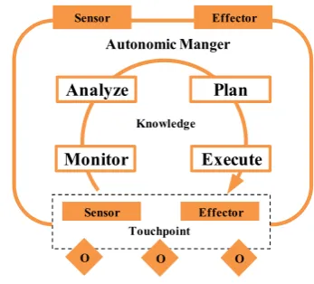
We leverage the well-accepted autonomic control loop pro-posed in IBM’s autonomic computing white paper [2] to be the basic model of adaptive computation. As shown in Fig.1, a control loop includes four abstract autonomic func-tions: (1) monitor, which collects data from managed ob-jects, e.g., the thread-pool states of a JEE server; (2)analyze, which processes and analyzes the collected data to deter-mine whether a system change is necessary, e.g., all threads are busy and there are still waiting business requests, thus new threads should be created for processing the waiting requests; (3)plan, which makes a proper plan of changing based on the analysis results, e.g., create five new threads into the thread-pool; (4) execute, which puts the plan into practice. The data shared by these functions are stored as knowledge that includes rules, history data, etc. An auto-nomic manager manages the objects by actually executing the adaptive computation in accordance with such a control loop. The manager retrieves data from the managed object throughsensorinterfaces, and changes the behavior of the object through effector interfaces. A touchpoint helps the autonomic managermap manageability interfaces to the ob-ject’s implementations. An autonomic manager itself also provides thesensorandeffectorinterfaces that can be used by a high level orchestratingautonomic managerto manage its states and behaviors. Therefore, it is possible to use an orchestrating autonomic managerto tune the execution of multiple sub-levelautonomic managers.

3_{http://java.sun.com/developer/earlyAccess/j2ee/ecperf/}

download.html. 4_{http://rubis.ow2.org.}

Fig. 1 The autonomic control loop

Adaptive computation (AC) is the abstract representation of the autonomic control loop described above. While a so calledmatureAC [2] should include all the four functions in the loop, other ACs can include only parts of the four functions. For instance, a JEE server such as PkuAS pro-vides several JMX MBean services [29] that expose the in-ternal states of the server and the hosted applications in its management console. Such a service can be considered as an AC with only themonitorfunction. Another case is LTA (the “Log/Trace Analyzer,” a component in the IBM auto-nomic computing toolkit: Tivoli), which can be considered as an AC withmonitorandanalyzefunctions.

Theautonomic level[2] of an AC refers to themaximum allowedcompletion level in the current iteration of its con-trol loop. For instance, if LTA is allowed to run only the monitor function in an iteration of its control loop, and is allowed to run through all the two functions (i.e.,monitor andanalyze) in the next iteration, we say that the autonomic level of LTA in the former case islowerthan that in the lat-ter case. The level-changing from the former to the latlat-ter is calledupgrade, otherwise,degrade. Upgrading the auto-nomic level of an AC is usually accompanied byincreased resource consumption because more functions can be run, while degrading the level is usually accompanied by de-creasedresource consumption.

2.2 A motivating example

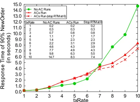
Fig. 2 The ECperf results of PkuAS running with and without ACs

then send an alarm to administrators. TPA dynamically ad-justs the thread-pool size of PkuAS in accordance with re-sponse time and throughput [10].

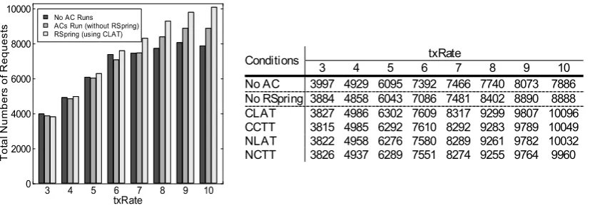
ECperf [33] is a JEE benchmark application. Its EJB components perform the typical e-business transactions (e.g., products-browsingandordering). Its test driver sim-ulates client requests to ECperf’s EJBs deployed in a JEE server. The driver has an adjustable integer parame-ter called txRate, which deparame-termines the requests generation rate. 1 txRate can be considered as 1,000 transactions per minute approximately. Thus, the workload increases with the increase of txRate.

We setup the following tests to see that if ACs can really interfere with the processing of business functions when the available resources are limited and competed. The testing environment is: the PkuAS hosting ECperf, the test driver, and the Oracle 9i database used by ECperf are each running on a machine with Ubuntu 8.04; Intel Core Duo 1.66 GHZ; 2 GB; and 100 Mb/s. We use the txRate from 1 to 10 to get the “response time of 90 % NewOrder,” which is the most important test index of ECperf. Figure2 presents the test-ing results. In this figure, “No AC Runs” denotes the “pure” PkuAS running with no ACs. “ACs Run” denotes PkuAS running with TPA, LP, and RTM. Each of the three ACs is executed always at its highest autonomic level in this test. That is to say, TPA and LP stick to run through all the four functions in each iteration of the autonomic control loop, and RTM runs with the singlemonitor function being exe-cuted. “ACs Run (stop RTM at 6)” denotes that we manually stop RTM when txRate≥6.

When txRate is 1 and 2, the available resources are rel-atively abundant with regard to the resource needs of ACs and business functions at the given workloads. Thus, we get the same “response time of 90 % NewOrder” results in the “No AC Runs” and “ACs Run” tests. However, when txRate is above 3, the resources become scarce at the given work-loads. In such cases, the ACs indeed compete with business

functions for the limited resources, which will surely inter-fere with the processing of the latter. For instance, when txRate is 6, the tested result in “ACs Run” is 141 % of that in “No AC Runs” test.ACs can incur performance penal-ties, but being a full-fledged autonomic JEE server, PkuAS needs to run together with them.For instance, LP manages logs and RTM records response time for administration. As to TPA, what should be noted is that it manages the thread-pool of PkuAS, which can improve the system performance if the management effects exceed the runtime costs. That is why we see in Fig.2 that when txRate is above 6, the performance of PkuAS running with ACs is much better than that of the “pure” PkuAS. The “ACs Run” curve also illustrates the main use of ACs: self-handling unexpected extreme cases such as a sudden surge of client requests or runtime exceptions.

The test of “ACs Run (stop RTM at 6)” in Fig.2proves the worth of degrading or stopping thenoncriticalACs to support system performance when necessary, that is, de-grade or stop the ACs that contribute little to system per-formance improvement, and meanwhile have little impact on the correct execution of the system if being degraded or stopped. The curve shows that the system performance in this case is even better than that of the “ACs Run” test when txRate≥6. For instance, when txRate is 10, the re-sponse time of “90 % NewOrder” is 10.8 % lower, which is a great improvement when under such a heavy work-load. However, the manual tuning way may be ineffective to achieve timely response to varying workloads. Therefore, an automatic tuner is necessary.

In addition, different ACs should be treated differently when being tuned. Each AC has its own specific features and usually produces different gains with regard to system performance. For example, if PkuAS does not run with TPA, its performance could be poorer most of the time than run-ning with TPA together. TPA can produce greater gains and is more cost-effective than the other two ACs with regard to system performance. Thus, it should better be run or its au-tonomic level should be upgraded first if resources are avail-able to do so. On the other hand, when executed under an ex-tremely heavy load, TPA may be less effective than in usual cases. Because only adjusting the thread-pool cannot mit-igate the increasingly fierce resource competition between business functions and ACs, and cannot offset the deteri-oration of system performance caused by the heavy work-loads. In such a case, a better strategy can be to degrade or stop TPA for devoting its resource-holdings to business functions. Thus AC tuning should have a global view, and should consider the specific features and gain of each AC.

3 Tuning model

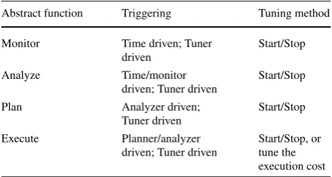
Table 1 Tuning an AC

Abstract function Triggering Tuning method Monitor Time driven; Tuner

driven

Start/Stop

Analyze Time/monitor

driven; Tuner driven

Start/Stop

Plan Analyzer driven;

Tuner driven

Start/Stop Execute Planner/analyzer

driven; Tuner driven

Start/Stop, or tune the execution cost

by upgrading and degrading the autonomic levels of ACs dy-namically. The model considers the features and gain of an AC. Based on the model, the RSpring tuner is implemented for tuning the ACs of an autonomic JEE server when re-sources are limited and competed.

3.1 The features of an adaptive computation

An AC includes either the completed autonomic control loop (see Fig.1), or just one or more functions in the loop (i.e., monitor, analyze, plan, or execute). Table 1 lists the tuning methods used in our model for the four abstract au-tonomic functions that can exist in an AC. In this table, trig-gering denotes in what condition or by which driving-force the functions can be trigged to run or stop, and this table lists the general triggers of each function (e.g., time-driven denotes themonitorfunction will be driven to run at a partic-ular point in time or at regpartic-ular intervals). Other triggers such as event driver or message driver are much more application and context specific (thus not be shown in the table), but they still conform to the tuning methods described below.

We can see from Table1that the tuning methods for mon-itor,analyze, andplanfunctions are start or stop, while for executefunction are start, stop, and tune the execution cost. Of course, these methods can be refined to include more types, e.g., themonitor function can have a tuning method for changing its running cost, which is similar to theexecute function. However, adding more methods will not alter the basic tuning mechanism: degrade or stop an AC for spar-ing system resources, and upgrade or run it for makspar-ing full use of resources. Similarly, although the four functions in Table1 can also be refined, it will make the tuning model too specific. The four-function autonomic control loop has already been widely accepted and practiced in both indus-try and academia [3,4]. Thus, the functions and methods in Table1 are sufficient to illustrate the tuning mechanism and suitable for modeling the different ACs that exist in JEE servers. Take the RTM of PkuAS as an example (Sect.2.2), its providedResponseMonitoringfunction is modeled as the abovemonitorfunction. ThestartListeningand stopListen-ingmethods of itsRTMServiceMBeaninterface are modeled

Table 2 The valid states of an AC State Definition

S0 All the four autonomic functions in the control loop are stopped

S1 Only themonitorfunction is started S2 S1is true and theanalyzefunction is started S3(E0) S2is true and if a change is necessary, theexecute

function is started

as the start/stop methods for this function. What should be noted is that, as a control loop, if themonitor function is stopped, the tuning of other functions will have no effect. When themonitorfunction is started and theanalyze func-tion is stopped, there is no need to tune theplanor the exe-cutefunction. Thus, the valid states of the control loop that an AC runs through can be defined in Table2.

As mentioned in Sect.2.1, not all the four functions must exist in an AC, thus an AC may only have parts of the states listed above. In addition, there are two issues to note in Ta-ble2: (1) it does not have a separate state to represent the planfunction. Because the separation of the four functions in the autonomic control loop is only a logical one, and a survey [4] shows that many ACs rarely implement a sepa-rateplanfunction (due to the fact that it is too costly to im-plement a fully automaticplanfunction, or theplanand the analyzefunctions are usually implemented as a whole, that is, a monolithic analyzefunction). Therefore, for simplic-ity’s sake, we omit theplan-related states; (2) the S3state in Table2 can be further divided into substates such as E1to Enaccording to different execution costs, wherendepends on the concrete control loop.

Theautonomic levelof an AC is identified by thehighest stateallowed to occupyin an iteration of its loop. In gen-eral, being the abstract representation of a control loop, the resource costsof an AC in different levels can be sorted in ascending order as follows:

S0<S1<S2<S3(E0) <E1<· · ·<En

If the level of an AC is changed in the left-to-right or-der in accordance with the above inequality, we call it up-grade, otherwise, degrade. Tuning (i.e., upgrading or de-grading) the level of an AC is implemented as setting a properhighest allowed statefor the corresponding control loop. To simplify the work of the RSpring tuner, we assume that the execution-costs of an AC (i.e., the resource costs re-lated to the states ranging from E1to En) are adjusted by the AC itself, thus RSpring only switches the states between Si (i∈ [0,3]).

be “natively” tuned at the four different autonomic levels, i.e., S0, S1, S2, and S3. Thus, dynamically upgrade/degrade the levels of ACs can be leveraged to tradeoff business func-tions and ACs for guaranteeing system performance when resources are limited and competed. The following two facts further ensure its possibility and feasibility. First, many ACs, especially those for monitoring and analyzing purposes, can be carried out without real-time constraints [2]. In other words, it is unnecessary to perform these computations at predetermined or fixed intervals, or complete them at a par-ticular point in time. For the mature ACs, if the execute function is stopped, its monitor andanalyze function can still work, and the data being collected or preprocessed by these two functions can be further processed when the exe-cutefunction is started [2–4]. That is to say, an AC currently with a relatively lower autonomic level can be upgraded by running more functions in the future iteration of the control loop, and thus consumes more system resources. Therefore, it is possible to bring about flexible resource costs with rel-atively little negative impact on ACs by upgrading or de-grading them dynamically. Second, the varying workloads, usually experienced by a JEE system, support the dynamic execution of ACs. When the workload is relatively low or within an acceptable range, it is reasonable to start running the ACs and upgrade them to make full use of resources. On the contrary, when the workload stays very high, it is feasi-ble to stop thenoncriticalACs (e.g., the RTM in Sect.2.2) or degrade them to save resources for processing more busi-ness requests. Of course, the running of thosecriticalACs (e.g., the one for self-healing and self-protecting) should be guaranteed even if the total available resources are limited. We will describe how to deal with such a case in detail in the next section.

3.2 The gain of an adaptive computation

To tune multiple ACs, the relative importance and cost-effectiveness of them should first be identified. We define the gain of an AC to be the positive impacts with regard to system performance, which are brought by the execution of an AC under a given amount of resources. We leverage the gain values to compare different ACs. What should be noted is that: The gain of an AC is not limited to system performance, but may include other benefits such as secu-rity enhancing or reliability improving. However, since the basic goal of our work is to guarantee performance when resources are limited and competed, we consider only the gains regarding performance. The gain value of an AC is di-rectly proportional to the positive impacts (e.g., throughput increasing) brought by this AC for business function pro-cessing, and is inversely proportional to the side effects for the correct execution of the whole system (e.g., error in-creasing). In our model, these values are only used to

com-pare different ACs for tuning the most suitable one, but not for exactly evaluating an AC.

Generally speaking, an AC with a higher gain should be degraded, in frequency and extent, less than that with a lower gain. Of course, there is such a possibility that an AC never wants its level to be tuned (e.g., the critical one for fault tolerance) even if it already has a very high gain value. In such cases, our tuning model allows an AC to specify a pinnedLevelSi (i∈ [0,3]). Once reaching thepinnedLevel, any tuning operations on the AC will have no effect. Our model also defines theminLevelSi (i∈ [0,3]) due to that some ACs can only be degraded to a specific lowest level. Therefore, if such an AC is degraded, its level cannot be lower than theminLevel. In addition, the importance of an AC to the system performance often relies on the states of the managed objects, and thus changes at runtime. For instance, garbage collection [28] will become much more important and produce greater gains when free memory is unavailable, and fault tolerance should be applied immedi-ately if a critical error happened. Therefore, to prevent bring-ing unexpected negative effects to an AC bebring-ing tuned, our model introduces the concept ofSafeRange. We assume that each managed object has an associatedSafeRangethat can be expressed as something like: “the ratio between the free threads and the total threads in the thread-pool should be higher than 5 %.” If an AC is found that the current state of its managed object exceeds theSafeRange, RSpring will stop tuning the AC for some time, and thus the AC can up-grade or deup-grade by itself to get back to theSafeRange.

Our work supports two ways to obtain the gain values: (1) Automatic. To be specific, the automatic ways to ob-tain the gain values are many. One often used is profiling. Online profiling can obtain dynamic gain values, but its run-ning cost is very expensive. Offline profiling is more suitable in the context our work targeted. However, it still requires much preparatory work such as probe-like instrument. What should be noted is that, RSpring leverages only the results of profiling (i.e., a sequence of ACs with comparable gain val-ues). Thus the profiling itself is not our focus. In addition, our work has another way to assign the gain values based on an AC’smaturity[2] (which implies the importance and cost-effectiveness of the AC to the whole system). For in-stance, if an AC has all the four functions of the autonomic control loop, while another AC has only themonitor func-tion, the former will be assigned a bigger gain value than the latter. (2) Manual. It requires administrators to assign the gain values, because they are the best candidate to know which AC can contribute most to system performance and to what extent. Such labor-based work is not much and not difficult, because the gain values are used for comparison, which can be assigned approximately.

managed object of ACq. Ifq is degraded, its managed ob-ject may be cleaned or closed without notifying p, which may cause exceptions inp. In such cases,pinnedLeveland minLevelcan be assigned to preventqfrom being tuned. The other relationship is that an ACpuses the autonomic func-tions of ACq, e.g.,monitor. If themonitorfunction ofqis stopped,pwill be affected. Although in our previous work [24], we find that there is no such function-sharing cases in the investigated JEE servers, e.g., PkuAS and JOnAS, the tuning model uses the following strategy to address this is-sue. That is, when an AC is tuned and the tuning requires stopping an autonomic function that is shared by another AC, the level of the formal AC is just degraded without stopping the shared function. In a JEE server, the above two relationships among ACs are often well documented in sys-tem manuals such as the JOnAS v5 configuration guide [32]. Therefore, they can be identified with relatively little effort by referring the manuals.

4 The RSpring tuner

We present RSpring for autonomic JEE servers. It is short for “Resource Spring,” which means the tuner is act as a “spring” to control the resource quotas between business functions and ACs. RSpring implements several tuning al-gorithms to decide when and to what extent an AC can be tuned. These algorithms are designed by referring to the OS process scheduling [25] with emphasis on the following is-sues:

• AC tuning is similar to process scheduling, but they have something in difference. First, process scheduling is to se-lect a process to consume resources (e.g., CPU), while AC tuning is to degrade (i.e., return some of the possessed re-sources) or upgrade an AC (i.e., consume relatively more resources). Second, a process has only the states related to stop/start, while an AC may have more states (i.e., S0, S1, S2, and S3). Thus, the process scheduling algorithms are not readily applicable in our work.

• Although some relatively complex AC tuning algorithms may be available, e.g., using feedbacks or Markov predic-tion, they usually cost much more runtime resources [26]. In a resource limited and competed environment, these resource-hungry algorithms should not be used, other-wise the whole system performance may become even worse [25,26]. We have had tested the Markov prediction scheduling algorithm in a trial experiment. The results are not good enough because the runtime overhead brought about by prediction will offset the tuning effects. In addi-tion, by referring to process scheduling, we find that all the scheduling algorithms are simple and effective. Our tuning algorithms are also inspired by them, which are representative, effective, and have a low overhead.

• The mechanism behind these algorithms is the same: en-able a flexible tradeoff between business functions and ACs by executing the latter dynamically when resources are limited and competed.

4.1 Two concerns in algorithm design

Priority The essence of AC-tuning is a scheduling prob-lem. In such a problem, priority is always the primary concern. For instance, the priority in the First-In-First-Out (FIFO) scheduling is the time of object-arriving. Even in the Round Robin scheduling, the priority of each scheduled ob-ject is implicitly considered (i.e., the priority values are the same). Therefore, the priority of each AC is also the primary concern in our tuning algorithms, and we use the gain value of each AC as its priority of tuning. Additionally, by consid-ering the features of an AC (Sect.3.1), the priority concern can be manifested at two representative granularity levels: the single state of AC (i.e., fine-grained) and the AC as a whole (i.e., coarse-grained). For instance, there are two ma-tureACs: L and H, and the gain of L is lower than that of H. “priority highlighted at AC state” means if L is degraded from S3to S2(i.e., in fine-grained)beforeH, then it will be upgraded from S2to S3afterH; “priority highlighted at AC” means if L is degraded from S3to S0(i.e., in coarse-grained) beforeH, then it will be upgraded from S0to S3afterH, al-though it may be upgraded from S0to S1beforeH.

Fairness The second important concern is fairness. How to manifest priority upon fairness is challenging. Also, use L and H as an example, if considering only priority, L will be degraded more and upgraded less than H. However, as de-scribed in Sect.3.2, the importance and cost-effectiveness of L may change at runtime. Although, thepinned-Level, min-Level, andSafeRangecan be used to address the dynamic gain issue, they cannot prevent the situation that: L will al-ways be degraded while H will alal-ways be upgraded. If we consider such a case is unfavorable, then how to apply fair-ness to prevent it happening? Similarly, by considering the features of an AC, our tuning algorithms apply fairness at two representative granularity levels: the single state of AC and the AC as a whole. Use L and H as an example again: “fairness highlighted at AC state” means if L is degraded from S3to S2(i.e., in fine-grained)beforeH, then it will be upgraded from S2 to S3 beforeH; “fairness highlighted at AC” means if L is degraded from S3 to S0 (i.e., in coarse-grained)beforeH, then it will be upgraded from S0 to S3 beforeH, although it may be upgraded from S0 to S1 af-terH.

Fig. 3 The autonomic-level changing diagram of ACs (“H” with a high gain and “L” with a low gain) by using different tuning algorithms

Fig. 4 The CLAT algorithm (the default tuning algorithm of RSpring)

same algorithm: if an AC is being degraded, it will never be degraded again until the other ACs with higher gains are de-graded. For another instance, in the NLAT algorithm where fairness is highlighted at the granularity of AC state, prior-ity is also manifested: an AC with a high gain value will be degraded after the AC with a low gain value (please see the next section).

4.2 Algorithms in detail

4.2.1 Covered load-amortizing tune (CLAT): the default algorithm of RSpring

CLAT is an algorithm in which “priority” is highlighted at the granularity of “AC State.” It is presented in Fig.4. The algorithm supports the following tuning features:

1. Controlled by RSpring, an AC with a high gain value is upgraded before and degraded after those ACs with rela-tively low gain values.

2. If an AC is upgraded by RSpring, the new level of this AC must be lower than or at most equal to the lowest level of those ACs with higher gain values; and if an AC

is degraded by RSpring, the new level of this AC must be higher than or at least equal to the highest level of those ACs with lower gain values.

3. RSpring must not upgrade/degrade the same AC again until it upgrades/degrades all the other ACs. This feature will not work when theSafeRangeconstraint of an AC is violated (Sect.3.2) and meanwhile the results of the self level-changing conflict with the above two features.

The details of the CLAT Algorithm are as follows

Data structure: Two double-ended queues (abbreviated to deque) that are used to contain ACs:

• remainDeque: contains the ACs that have not been tuned since the last time the algorithm is executed. • changedDeque: contains the ACs that have been

tuned since the last time the algorithm is executed. Input:

All these ACs are copied to theremainDequein se-quence when initializing RSpring.

• A system load metric (e.g., CPU utilization) and the corresponding thresholds:lowerBoundand up-perBound(e.g., CPU utilization between 75 % and 85 %).

Helper methods:

• getCurLoad(metric): get the current system load measured by the given metric.

• calibrateACPos (tuningOperation):

ad-just the position of each AC in between the remain-Dequeand thechangedDequeaccording to an AC’s current level, gain value, and the tuning operation to be performed. This method is used to guarantee the tree tuning features of the algorithm. As described in Sect.3.2, an AC can upgrade or degrade by it-self without the control of RSpring when the state of the managed object exceeds its SafeRange, and thus may interfere with the three features. There-fore, calibration is necessary.

• inSafeRange (AC): given an AC, check if the state of the managed object is in itsSafeRange. • initialized(AC): check if an AC has been set

to its initial level.

• tuning (AC,tuningOp): upgrade, degrade, or initialize an AC.

• swap(Deque a,Deque b): swap the given two deques.

The CLAT algorithm is briefly explained as follows: Line 1: get the current system load (curLoad) according to a given load metric (e.g., CPU utilization).Line2∼21: if the curLoadis lower than the predefinedlowerBound, the algo-rithm will upgrade ACs in accordance with the three tun-ing features described above.Line 22∼38: if thecurLoadis higher than the predefinedupperBound, the algorithm will degrade ACs in accordance with the three tuning features. The complexity of the CLAT algorithm is O(n), where n is the number of ACs being tuned. Thus, it is affordable to run in a resource limited and competed environment (the run-time cost of CLAT will be shown in Sect.5).

The autonomic-level changing diagram of CLAT is shown in Fig.3(a). In this figure, H and L are both the so-calledmature ACs. H’sgain value is higher than L’s. We can see that the curve-changing patterns reflect the three tuning features of CLAT described above. In CLAT, “prior-ity” is highlighted at the granularity of “AC state.” Because

the curve of H covers the curve of L in every change (i.e., upgrade/degrade) of AC state. In addition, fairness is also manifested in CLAT due to H has to be degraded before L being degraded once again. That is why CLAT is named as: Covered Load-Amortizing Tune.

4.2.2 Covered carry-through tune (CCTT)

CCTT is an algorithm in which “priority” is highlighted at the granularity of “AC.” It is presented in Fig.5. The algo-rithm supports the following two tuning features:

• Controlled by the tuner, an AC with a highgainvalue is upgraded before and degraded after those ACs with rela-tively lowgainvalues.

• Before an AC being upgraded by the tuner, each of the other ACs with highergainvalues must have been up-graded to its highest level (e.g., S3), and all the other ACs with lower or equalgainvalues must not be tuned until the upgrading of the current AC to its highest level is fin-ished; before an AC being degraded by the tuner, each of the other ACs with lowergainvalues must have been de-graded to its lowest level (e.g., S0), and all the other ACs with higher or equalgainvalues must not be tuned un-til the degrading of the current AC to its lowest level is finished. This feature will not work when the SafeRange constraint of an AC is violated and meanwhile the results of the self level-changing conflict with the first feature. The details of the CCTT Algorithm are as follows The data structure, input, helper methods of CCTT are the same as that of CLAT in Sect.4.2.1. However, the calibrateACPos method has a different internal implementation, which is used to guarantee the two specific tuning features of CCTT. There are two additional helper methods in CCTT:

• isAtHighestLevel (AC): check if an AC has been set to its highest autonomic level.

• isAtLowestLevel(AC): check if an AC has been set to its lowest autonomic level.

The differences between CCTT and CLAT are: when up-grading, CCTT will explicitly check if the current AC being tuned is at its highest adaptive level (Line 12). If the check returns false, the current AC will prepare for the next round tuning by being pushed back to remainDequerather than always being added tochangedDequeas in CLAT. Similar characteristics can be found inLine 28when degrading is performed.

The autonomic-level changing diagram of CCTT is shown in Fig.3(b). We can see that the curve-changing pat-terns of H and L in this figure reflect the two tuning features of CCTT described above. We can also see that in CCTT, “priority” is highlighted at the granularity of “AC.” Because the curve of H remains at its highest level S3when the curve of L degrading from S3to S0, and because L can only be upgraded until H has been upgraded to its highest level (i.e., carry through). That is why CCTT is named as: Covered Carry-Through Tune.

4.2.3 Other algorithms

RSpring has implemented several other algorithms. For instance, the NLAT (Noncovered Load-Amortizing Tune) shown in Fig. 3(c) is similar to the CLAT algorithm in Fig.3(a). However, we can see that in NLAT, “fairness” is more highlighted than that in CLAT. Because the curve of L can be upgraded before the curve of H (i.e., the curve of H does not always cover that of L). That is why NLAT is named as: Noncovered Load-Amortizing Tune. For another instance, the NCTT (Noncovered Carry-Through Tune) in Fig.3(d) is similar to CCTT in Fig.3(b). Their main differ-ence is that in NCTT, “fairness” is highlighted at the gran-ularity of “AC.” Because in NCTT the curve of L can be upgraded before the curve of H, and because L will be graded all the way to its highest level before H can be up-graded.

The algorithms in Fig.3are all representative ones to de-cide when and to what extent an AC can be tuned. However, it is difficult to tell which algorithm is always better than others (see the experiments in Sect.5). For instance, when the upper bound of the system load is exceeded, whether RSpring should stop an AC immediately and completely (similar to CCTT and NCTT), or degrade two or more ACs in sequence (similar to CLAT and NLAT). This is an open issue. The reason behind is that the runtime effects of a tun-ing algorithm is affected by many factors, e.g., the system workload and the current autonomic-level of each AC. The detailed comparison of these algorithms is not the focus of this article and will be addressed in the future work.

4.3 The implementation of RSpring

PkuAS is built upon the JMX specification [29]. Its ACs are a set of MBean services. Thus, we implement RSpring also as an MBean service of PkuAS, so that it can get the states of the ACs and control their behaviors through MBean interfaces. JOnAS v5 is built upon JMX and OSGi [30]. Similarly, RSpring is implemented as a service of JOnAS. The other built-in services of JOnAS take the form of OSGi service bundles, which can be regarded as the ACs in our work. Thestop/startstates of aservice bundlecan be viewed

as the S0 and the Si (i∈ [1,3]) level of an AC, respec-tively. For instance, RSpring uses the stop/start methods of the “org.ow2.jonas.discovery.base.DiscoveryServiceImplM Bean” interface to tune the discovery service of JOnAS at the level of S0. The activation and deactivation of the OSGi/JMX methods supplied in such abundlehelp to re-fine the autonomic levels into the specific S1, S2, or S3. For instance, the “disableEJBLogger” and “enableEJBLogger” methods of “org.ow2.jonas.audit.logger.AuditLogCompo nentMBean” can be used to tune theauditservice of JOnAS from S0to S1and back forth.

In practice, we find that CPU/memory are the most criti-cal resources in competition between business functions and ACs in most cases [6,18,20,23]. The utilization of these resources can be used as indicators of system loads. There-fore, at present, RSpring supports CPU/memory utilization as a system load metric.

RSpring has its configuration file for PkuAS and JOnAS respectively. To make it work, several parameters should be assigned such as the controlled classes of the AC-compliant JMX/OSGi services identified by administrators, the spe-cific methods in these classes to tune the corresponding ACs at different autonomic levels, and the lower and upper bounds for system load metric. The upper bound should take into account the unpredictable burst of business requests. The gap between the lower and the upper bound should not be too large. Otherwise, very few ACs could be carried out simultaneously. On the other hand, to avoid CPU or memory thrashing, the gap should not be too small either. Therefore, to assign appropriate thresholds, the experience of a system administrator plays an important role, and should take into account the resources hold by the whole JEE system. Some trials are also necessary before assigning these parameters. The newest version of RSpring can be downloaded at the website of PkuAS.

5 Evaluation

We setup two experiments to evaluate the effectiveness of RSpring by using industry standard JEE benchmark appli-cations and autonomic JEE servers. The first experiment runs ECperf in PkuAS, and uses RSpring to tune the ACs of PkuAS described in the motivating example. The second runs RUBiS in JOnAS, and uses RSpring to improve the sys-tem performance by tuning the AC-compliant OSGi services of JOnAS.

5.1 ECperf+PkuAS 5.1.1 Experimental setup

Fig. 6 The response time results of ECperf when PkuAS running with and without RSpring

is assigned the lowest gain value, because it produces the lowest gains with regard to system performance comparing with the other two. RTM has only amonitorfunction, so its possible autonomic levels are S0and S1. LP’s possible lev-els are S0, S1, S2, and S3. TPA is assigned with the highest gain value. Thus, it is guaranteed to run or upgrade first if resources are available to do so. The levels of TPA are also S0, S1, S2, and S3. TPA has defined itsSafeRangeas be-low: the current busy threads should not exceed 95 % of all the threads in the thread-pool. If this constraint is violated, RSpring will stop tuning TPA for some time. Thus, TPA can upgrade or degrade by itself to get back to theSafeRangevia adjusting the thread-pool size.

The experiment setup remains unchanged as described in Sect. 2. The tested txRate of ECperf is from 3 to 10 and with the sequence 3, 5, 7, 9, 10, 8, 6, 4 to simulate heavy and varying workloads. Such a sequence (with the “normal distribution” pattern) can best simulate the most-appeared workloads in enterprise environment [27]. The testing time lasts 80 minutes. Every 10 minutes, the driver issues a new test with a new txRate. We use CPU utilization as the system load metric, because CPU is the most critical resource in the scenario of ECperf. The corresponding thresholds are set to 75 % (lower bound) and 85 % (upper bound) of CPU utilization, respectively.

5.1.2 Performance of ECperf

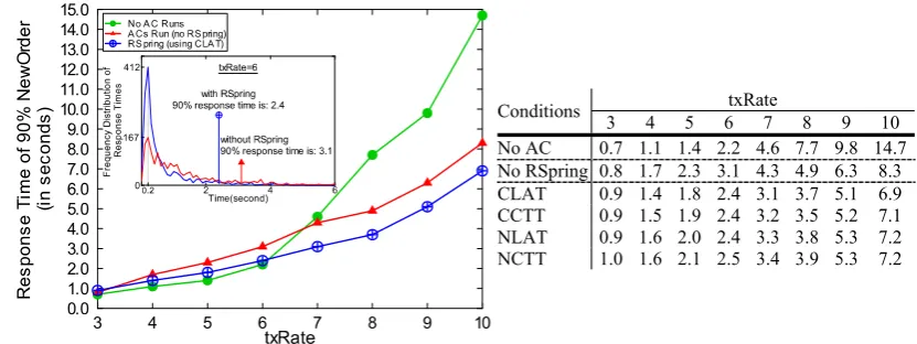
We compare the “response time of 90 % NewOrder” results of ECperf in the following three cases: (1) PkuAS runs with-out ACs, i.e., “pure” PkuAS; (2) it runs with all the three ACs described above; (3) and it runs with the ACs and also with RSpring. Figure6shows the results. In this figure, the tested txRate sequence is arranged in ascending order, so that we can compare it with Fig. 2, and show the effects of RSpring clearly. From Fig. 6, we can see that the re-sults of “RSpring” are generally much better than that of

the “ACs Run (no RSpring)” test. Additionally, the perfor-mance penalty of RSpring is quite small. For instance, when txRate is 6, the response time of “RSpring (using CLAT al-gorithm)” is 2.4, which is just 0.2 seconds higher than that of the “pure” PkuAS. We can get the same conclusion from the tests of RSpring using other algorithms. Being a full-fledged autonomic JEE server, PkuAS needs to run with ACs, and thus RSpring is also necessary to guarantee the performance of the whole system.

The frequency distribution of the NewOrder response times is as follows (see the figure inside Fig.6). If RSpring uses the default CLAT algorithm and when txRate is 6, there are 412 NewOrder transactions with their response times at 0.2 seconds. However, if PkuAS runs with ACs but with-out RSpring, the number of this kind of transactions is only 167. The average response time with and without RSpring are 0.983 and 1.572, respectively, and the “response time of 90 % NewOrder” are 2.4 and 3.1, respectively. These values indicate that RSpring indeed improves the system perfor-mance by tuning ACs.

other. We cannot tell which one is always better than others, but we can tell that they all bring better results than the tests of “ACs Run (no RSpring).” The reason behind is that all the algorithms reflect the same tuning mechanism: enable a flexible tradeoff between business functions and ACs by executing the latter dynamically when resources are limited and competed.

The autonomic-level changes of the three ACs in the case of PkuAS running with RSpring (using the default CLAT al-gorithm) are shown in Fig.7. We can see from this figure that with RSpring, the levels of the ACs change up or down continuously with the varying workloads, which bring about flexible resource costs. Without RSpring, however, the auto-nomic levels will stick to their original states all the time, thus incur an approximately fixed resource costs regard-less of the ever-changing workloads. In addition, Figs.7(a) and (b) show the two different changing patterns of the autonomic-level curves: no AC violates itsSafeRange con-straint and an AC violates itsSafeRangeconstraint.

• The curves in Fig.7(a) belong to the no-violation pattern. They have the following characteristics: (1) the TPA curve always decreases after and increases before the LP and RTM curves, while the RTM curve always behaves in the opposite way; (2) the TPA curve covers both the LP and

RTM curves all the time, and the LP curve always covers the RTM curve; (3) in a round of tuning, the TPA curve will not increase/decrease to a new level once more until the other two curves have both increased/decreased. Thus, we see that these characteristics reveal and conform to the three tuning features of the CLAT algorithm in Sect.4.2. • The TPA curve in Fig. 7(b) shows that TPA has

expe-rienced the violation of its SafeRange constraint when txRate is 7 (during the timeline of the 25∼27 and 28∼ 29 minutes). In such a case, RSpring will stop tuning TPA for a fixed time interval (e.g., 30 seconds). TPA will auto-matically adjust the size of the thread-pool (i.e., its man-aged object) for getting back to itsSafeRange, and thus it changes the autonomic level directly to S3by itself as shown in this figure.

As throughput is also an important indicator of system performance, we present the throughputs comparison be-tween PkuAS running with/without RSpring and without the three ACs (i.e., the “pure” PkuAS) respectively in Fig.8. We can see from this figure that the throughputs with RSpring are close to the ones without RSpring, and are also close to that of the “pure” PkuAS when txRate is relatively low (e.g., 3, 4, and 5). However, when txRate increases (e.g., 6, 7, 8, 9, and 10), the former becomes much higher than

Fig. 7 The autonomic-level changes of the three ACs when RSpring using the default algorithm

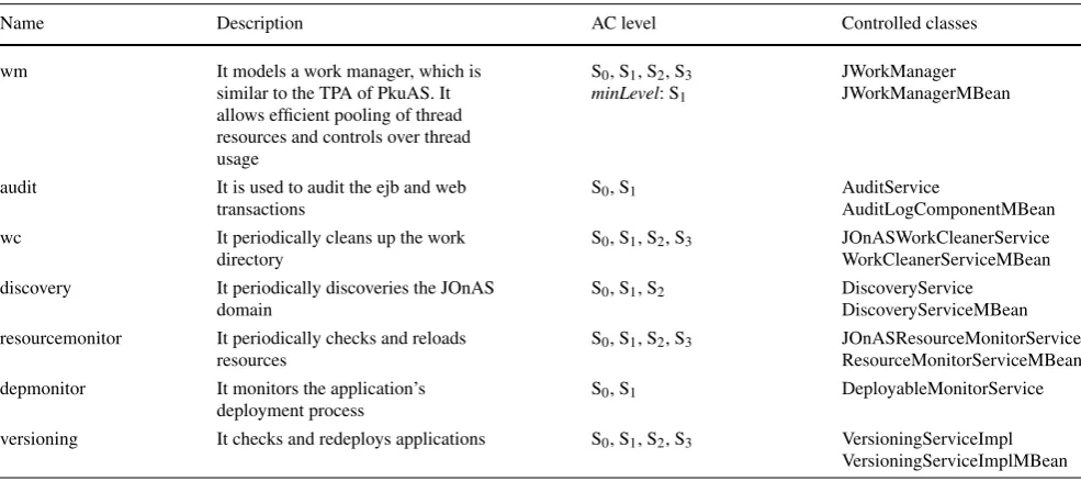
Table 3 The experimented AC-compliant OSGi/JMX services of JOnAS v5.2

Name Description AC level Controlled classes

wm It models a work manager, which is similar to the TPA of PkuAS. It allows efficient pooling of thread resources and controls over thread usage

S0, S1, S2, S3

minLevel: S1

JWorkManager JWorkManagerMBean

audit It is used to audit the ejb and web transactions

S0, S1 AuditService

AuditLogComponentMBean wc It periodically cleans up the work

directory

S0, S1, S2, S3 JOnASWorkCleanerService WorkCleanerServiceMBean discovery It periodically discoveries the JOnAS

domain

S0, S1, S2 DiscoveryService DiscoveryServiceMBean resourcemonitor It periodically checks and reloads

resources

S0, S1, S2, S3 JOnASResourceMonitorService ResourceMonitorServiceMBean depmonitor It monitors the application’s

deployment process

S0, S1 DeployableMonitorService versioning It checks and redeploys applications S0, S1, S2, S3 VersioningServiceImpl

VersioningServiceImplMBean

the latter two. For instance, when txRate is 6, the success-fully processed requests with RSpring (using CLAT) are 523 higher than that of “without RSpring” and 217 higher than that of the “pure” PkuAS. The differences increase to 1208 and 2210, respectively, when txRate is 10. That is to say, compared with PkuAS running with ACs,RSpring improves the system performance by 13.6 % with the same amount of resources. That is because the system resources such as CPU spared by degrading the ACs are used for processing more business requests, and thus brings higher throughputs. 5.2 RUBiS+JOnAS

5.2.1 Experimental setup

JOnAS [31] is an autonomic JEE server. It performs sev-eral AC-compliant OSGi/JMX services. In a JOnAS v5.2 instance, such services include wm,audit,wc, etc. For in-stance, the wm service of JOnAS is just like the TPA of PkuAS. It provides a facility to submit work instances for execution. The submitted work is carried out by a free work-thread in the thread-pool managed bywm. When there are waiting works and the current pool size does not exceed the max pool size,wm will automatically create a new work-thread to execute the waiting work. Always creating new threads in a resource limited and competed environment will intensify resource competition, and can sometimes make the system performance be even worse. Therefore, in such a case, wm should be tuned to degrade its autonomic level for sparing resources for business functions. However,wm has to be activated in most cases for the normal execution of the system. Thus, in our experiment,wm has the high-est gain value and defines itsSafeRangethat “maxPoolSize-curPoolSize ≥ 3 and maxWaitingTime(work) <60 s”, so

that it can be guaranteed to work if resources are avail-able and if itsSafeRangeis violated. Different to the TPA of PkuAS, thewmservice has defined itsminlevelto be S1 (see Sect.3.2), because it cannot be stopped due to the spe-cific requirement of theejb3service of JOnAS v5 [32]. For another instance, theaudit service logs the information of ejb transactions, which contains method name, process time, and method stack trace, etc. This service is like the RTM of PkuAS. RSpring for JOnAS will tune it by the start/stop, enableEJBLogger/disableeEJBLogger methods of the cor-respondingAuditLogComponentMBeaninterface. The other services participated in our experiment are shown in Ta-ble3.

test-Fig. 9 The performance results of RUBiS using theread-onlyrequest transition type.Error barsshow the standard deviation from the mean

Fig. 10 The performance results of RUBiS using theread-writerequest transition type.Error barsshow the standard deviation from the mean

ing results in this section just show RSpring using the de-fault CLAT tuning algorithm. The tests of the other algo-rithms can be found on the RSpring website, which can get the same conclusions as below.

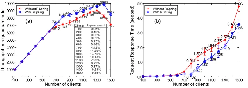
5.2.2 Performance of RUBiS

Figure9(a) shows the throughputs of RUBiS tested by the read-only type of request transitions. From this figure, we can see that when the workload is relatively low, e.g., 100 clients, the system performances with and without RSpring are almost the same. However, when the workloads become very heavy, the system performance with RSpring is much better. For instance, when there are 1400 clients, the range of the error bar for the throughput value in the “with RSpring” test does not overlap with that of the “without RSpring” test, andthe average throughput with RSpring is 19.23 % higher than that without RSpring. The autonomic-level change pat-terns of the ACs in JOnAS are similar to that shown in Fig.7, which can get the same conclusions as in the PkuAS ex-periment. The average response times of client requests are

shown in Fig.9(b). We can see that with RSpring, the re-sponse time is shorter than that without RSpring when the system load is heavy, and the error bar for the test with RSpring rarely overlap with that of the without RSpring test, which indicates the truly performance improvement of the system.

Figure 10 shows the performance of RUBiS when the clients performing the read-write type of request transitions. Similarly, we can find that with RSpring, RUBiS performs much better than that without RSpring;the throughputs im-provement can be as high as 11.7 %when there are 500 testing clients.

6 Related work

Our work, premised on the assumption that resources are limited and competed, supports a flexible tradeoff between ACs and business functions via the dynamic tuning of ACs. It belongs to the self-optimization category of system per-formance guaranteeing.

IBM WebSphere provides a mechanism to adjust the ap-plication execution environment according to a preferred usage profile [19]. Diao et al. [20] furnishes the Apache server with self-optimizing ability to keep CPU and mem-ory at a desire level by tuning two parameters of the server. Yang et al. [21] propose a profile-based approach to devel-oping just-in-time scalability for JEE applications. In this approach, expert’s knowledge of application scaling is cap-tured as profiles. Guided by profiles, an AC-like profiling driver automates the scaling of applications to ensure per-formance and improve resource utilization, e.g., increases or decreases the EJB instances constituting a JEE application. Although these works use ACs to satisfy end user’s needs or achieve a desired system state, they ignore the costs of ACs. Our work can be referred to as a self-optimization mecha-nism by considering the costs of ACs together.

Several studies on AC have considered performance penalty [22,28]. For instance, the JVM garbage collector takes performance cost of garbage collection into account by delaying collection or collecting only parts of the un-reachable objects at a time. Such kinds of self-optimization are at a low level and inside ACs, while our approach con-siders self-optimization at a relatively high level and among ACs. These two approaches are complementary and can be combined into the design of JEE servers.

In the research of runtime verification, probes are instru-mented into the programs being verified. Such a probe can capture and send back the interested events occurred dur-ing the execution of the program. To reduce the cost of dy-namic analysis, studies such as [13] exploit the results of static typestate analyses to reduce the number of probes and the amount of information to be recorded. Thus, we can view the probes as the monitor-level ACs, which can be tuned by RSpring.

A utility based approach has been used for allocating resources among different computations [8,14]. The main idea is to first use a utility function to express the rela-tionship between high level business goals and system per-formance, then use an empirical model to correlate system performance with resources allocation, and finally combine these two functions for representing a utility model that guides the allocation of resources. The main difficulty of ap-plying such an approach is to obtain the empirical model that exactly represents the relationship of resource allocation and performance. In addition, the runtime resource costs of the utility functions are usually high [14]. Therefore, our work

does not use utility functions for tuning ACs at present, es-pecially when targeting a resource limited environment.

Several studies such as [7, 15,16] try to guarantee the overall system performance by upgrading and degrading the service levels of business functions. When the system load is heavy, these functions will degrade their service levels for achieving a steady and high throughput, e.g., return the top 100 search results to a client instead of all the results, return the results without sorting, or just decrease the search qual-ity. Studies such as [17] leverage admission control to guar-antee high system performance. The application will refuse to serve any new incoming client requests when the system is under heavy stress. Other studies such as [18] schedule incoming requests to the order in which concurrent requests can be served. For instance, the application will distinguish the type of client requests and will first serve the ones with the shortest remaining processing time. In this way, more re-quests can be served. All the above approaches require the applications to be modified or built from the start to have the capability of dynamic service-level negotiation. Our ap-proach changes the levels of ACs instead of business func-tions, and thus leaves the business logic intact.

7 Conclusion and future work

With the increasing use of autonomic computing technolo-gies, JEE servers are implemented with more and more adaptive computations. It brings challenges to resource al-location for achieving the performance goals because of re-source competition between business functions and adap-tive computations, especially when the whole system is un-der heavy load. In this article, we have presented a tuning model for the performance improvement of applications in JEE servers. This model is built on the autonomic control loop, and the features and gain of an adaptive computation have been considered in the model. Based on the model, the autonomic level of an adaptive computation is upgraded or degraded dynamically so as to control its resource cost. We have implemented the RSpring tuner for JEE servers such as PkuAS and JOnAS, which has been evaluated by ECperf and RUBiS benchmark applications respectively. The results show that RSpring can effectively improve the application performance by 13.6 % in PkuAS and 19.2 % in JOnAS with the same amount of resources.

Acknowledgements The authors would like to thank all the anony-mous reviewers for their valuable comments and suggestions to im-prove the quality of the article. This work is supported by the Na-tional Basic Research Program of China (973) under Grant Nos. 2009CB320703; the National Natural Science Foundation of China un-der Grant No. 61121063, 60933003; the High-Tech Research and De-velopment Program of China (863) under Grant No. 2012AA011207; and the IBM University Joint Study Program.

References

1. IBM, Autonomic computing: IBM’s perspective. http://www. research.ibm.com/autonomic

2. IBM (2006) An architectural blueprint for autonomic computing. IBM White Paper

3. Dobson S, Sterritt R, Nixon P, Hinchey M (2010) Fulfilling the vision of autonomic computing. IEEE Comput 43:35–41 4. Salehie M, Tahvildari L (2009) Self-adaptive software: landscape

and research challenges. ACM Trans Auton Adapt Syst 4:1–42 5. Zhang Y, Huang G, Liu X, Zheng Z, Mei H (2010) Towards

auto-matic tuning of adaptive computations in autonomic middleware. In: 9th workshop on adaptive and reflective middleware (ARM), collocated with middleware

6. Zhang Y, Huang G, Liu X, Mei H (2010) Integrating resource con-sumption and allocation for infrastructure resources on-demand. In: Proceedings of the 3rd international conference on cloud com-puting

7. Philippe J, De Palma N, Gruber O (2009) Self-adapting service level in java enterprise edition. In: 10th international middleware conference (middleware)

8. Costa P, Napper J, Pierre G, van Steen M (2009) Autonomous re-source selection for decentralized utility computing. In: Proceed-ings of the 29th international conference on distributed computing systems (ICDCS), pp 561–570

9. Mei H, Huang G (2004) PKUAS: an architecture-based reflective component operating platform. In: The future trends of distributed computing systems, pp 163–169

10. Huang G, Liu T, Mei H, Zheng Z, Liu Z, Fan G (2004) Towards autonomic computing middleware via reflection. In: Proceedings of the 28th annual international computer software and applica-tions conference (COMPSAC)

11. Liu T, Huang G, Fan G, Mei H (2005) The coordinated recovery of data service and transaction service in JEE. In: Proc of COMP-SAC

12. Mei H, Huang G, Li J (2008) A software architecture centric self-adaptation approach for internetware. Sci China Ser 51(6): 722– 742

13. Dwyer MB, Purandare R (2007) Residual dynamic typestate anal-ysis exploiting static analanal-ysis: results to reformulate and reduce the cost of dynamic analysis. In: Proceedings of the twenty-second

IEEE/ACM international conference on automated software engi-neering (ASE). ACM, New York, pp 124–133

14. Walsh WE, Tesauro G, Kephart JO, Das R (2004) Utility func-tions. In: Autonomic systems, international conference on auto-nomic computing, pp 70–77

15. Mills RT (2004) Adapting to memory pressure from within ap-plications on multi-program COWs. In: International parallel and distributed processing symposium (IPDPS)

16. Chandra S, Ellis C (2000) Application-level differentiated web services using quality aware transcoding. IEEE J Sel Areas in Commun 18:2544–2565

17. Welsh MD (2002) An architecture for highly concurrent, well-conditioned internet services. PhD Thesis, UC Berkeley 18. Schroeder B et al (2006) Web servers under overload: how

scheduling can help. ACM Trans Internet Technol 6(1):20–52 19. Candea G, Kiciman E (2003) JAGR: an autonomous

self-recovering application server. In: Autonomic computing workshop on active middleware services

20. Chess YD, Hellerstein JL, Parekh S, Bigus JP (2003) Managing web server performance with autotune agents. IBM Syst J 42:136– 149

21. Jie Y, Jie Q, Ying L (2009) A profile-based approach to just-in-time scalability for cloud applications. In: IEEE international con-ference on cloud computing, pp 9–16

22. White SR, Hanson JE et al (2004) An architectural approach to autonomic computing, In: International conference on autonomic computing (ICAC), pp 2–9

23. John LK, Vasudevan P (1998) Workload characterization: motiva-tion, goals and methodology. In: Workload characterization work-load methodology and case studies

24. Chen X, Huang G (2010) Service encapsulation for middleware management interfaces. In: International symposium on service oriented system engineering, pp 272–279

25. Bruker P (2007) Scheduling algorithms, 5th edn. Springer, Berlin 26. Blazewicz J, Lenstra JK, Rinnooy Kan AHG (2007) Scheduling

subject to resource constraints: classification and complexity. Dis-crete Appl Math 5:11–24

27. Microsoft, patterns and practices: performance testing guidance.

http://perftesting.codeplex.com

28. Goetz B (2003) Java garbage collection in the HotSpot JVM, IBM developer Works

29. JMX (2011) Java Management eXtensions. http://jcp.org/jsr/ detail/77.jsp

30. OSGi Open service gateway initiative.http://www.osgi.org

31. JOnAS, The ObjectWeb next generation application server.http:// jonas.ow2.org

32. JOnAS configuration guide.http://jonas.ow2.org/JONAS_5_2_0/ doc/doc-en/pdf/configuration_guide.pdf

33. ECperf. http://java.sun.com/developer/earlyAccess/j2ee/ecperf/ download.html