Understanding predictability and exploration in human mobility

R E G U L A R A R T I C L E

Open Access

Understanding predictability and

exploration in human mobility

Andrea Cuttone

_{, Sune Lehmann}

_{and Marta C. González}

*_{Correspondence:}

andreacuttone@gmail.com

1_{DTU Compute, Technical University}

of Denmark, Richard Petersens Plads Building 324, Kgs. Lyngby, Denmark

3_{Department of Civil and}

Environmental Engineering and Engineering Systems, Massachusetts Institute of Technology, 77 Massachusetts Avenue, 1-290, Cambridge, 02139, United States

Full list of author information is available at the end of the article

Abstract

Predictive models for human mobility have important applications in many fields including traffic control, ubiquitous computing, and contextual advertisement. The predictive performance of models in literature varies quite broadly, from over 90% to under 40%. In this work we study which underlying factors - in terms of modeling approaches and spatio-temporal characteristics of the data sources - have resulted in this remarkably broad span of performance reported in the literature. Specifically we investigate which factors influence the accuracy of next-place prediction, using a high-precision location dataset of more than 400 users observed for periods between 3 months and one year. We show that it is much easier to achieve high accuracy when predicting the time-bin location than when predicting the next place. Moreover, we demonstrate how the temporal and spatial resolution of the data have strong influence on the accuracy of prediction. Finally we reveal that the exploration of new locations is an important factor in human mobility, and we measure that on average 20-25% of transitions are to new places, and approx. 70% of locations are visited only once. We discuss how these mechanisms are important factors limiting our ability to predict human mobility.

Keywords: human mobility; next-location prediction; predictability

1 Introduction

Billions of personal devices, ranging from in-car GPS to mobile phones and fitness bracelets, connect us to the cloud. These ubiquitous interconnections between the physi-cal and the digital world open up a host of new opportunities for predictive mobility mod-els. Each user of a device produces rich information that allows us to measure their daily mobility routine. This type of knowledge, especially when arising from large numbers of individuals, is expected to impact a wide range of areas such as health monitoring [1], ubiquitous computing [2, 3], disaster response [4], or smart traffic management [5]. Re-cent contributions to mobility modeling come from computer science [6–8], transporta-tion engineering [9, 10], geographic informatransporta-tion sciences [11, 12], and complexity sciences [13–15]. The state-of-the-art for mobility modeling has developed rapidly over the past decade, but further work is needed, especially to tackle the problem of individual pre-dictability.

In the literature, human mobility has been studied using a multitude of proxies (for ex-ample call detail records (CDR), GPS, WiFi, travel surveys), and a variety of techniques

have been suggested for predictive models, such as Markov chains, Naive Bayes, artifi-cial neural networks, time series analysis. Studies report varying results for the predictive power of these models, with accuracy from over 90% to under 40%.

In this paper we set out to uncover the reasons behind these surprisingly large differ-ences in performance via a systematic investigation of the factors that may influence esti-mates of mobility predictability. The key contributions of this paper are:

1. We investigate which factors influence performance in the reported cases of predictability. Showing that the differences in results are driven by the following questions: (a) Does the analysis concern anupper boundof predictability, or actual next-place prediction? (b) How is the prediction problem formulated? E.g. is the goal to predict the next location, or is the goal to identify location in the next time-bin? (c) What is the spatial resolution of the data source? E.g. is the analysis based on GPS vs. CDR data? (d) What is the temporal resolution of the data source e.g. minutes, hours?

2. We quantify the amount of explorations and locations visited only once, and show that these are key limiting factors in the accuracy of predictions for individual mobility.

3. We measure the predictive power of a number of contextual features (e.g. social proximity, time, call/SMS).

4. We study the problem of predictability of human mobility using a novel, longitudinal, high-precision location dataset for more than 400 users.

The rest of the paper is organized as follows. We first provide an overview of related work in the field of predictions of human mobility. Next, we introduce the dataset and describe the preprocessing steps. In the subsequent section we describe the baseline models, and compare their performances. Finally we introduce the exploration prediction problem and report the performance of the predictive models.

2 Related work

In a seminal paper Songet al. [13] investigate the limits of predictability of human mobility, using Call Detail Records (CDR) as proxy for human movement. In their analysis, the authors discretize location into a sequence of places, and estimate an upper limit for the predictive performance using Fano’s inequality on the temporal entropy of visits. Their results show that for a majority of users, this upper bound is surprisingly high (93%). This framework has been further explored to refine the estimate of the upper limit. Specifically, Lin et al. [16] study the effects of spatial and temporal resolution on the predictability limit, Smith et al. [17] consider spatial reachability constraints when selecting the next place to visit, and obtain a tighter upper bound of 81-85%, and Lu et al. [4] analyze the predictability of the population of Haiti after the earthquake in 2010, and find an upper limit of predictability of around 85%. The work described above focuses on estimating an upper limit of predictability for an individual based on an estimate of the entropy their trajectory.

authors apply the Markov models to WiFi traces at Darthmouth campus and find that the best performing model is order 2 and has a median accuracy of about 65-72%. Krumme et al. [20] applied Markov models on shopping locations inferred from credit card transac-tions, and found that models trained on the aggregate data from a large number of people perform better than individual models. Bapierre et al. [21] applied a variable-order Markov chain to the Reality Mining [6] and Geolife [22] datasets.

Another frequently used type of prediction framework is based on naive Bayes mod-els, where the probability of next location is factorized as independent probabilities for a number of context variables. Gao et al. [23] applied this approach to the Nokia Data Challenge dataset [24] using time and location features, and obtained an accuracy of ap-proximately 50%. Do et al. [25] applied the same technique but used a larger number of features including also SMS, calls and Bluetooth proximity, and obtained an accuracy of approximately 60%. In a subsequent paper [26] the same authors explore a kernel density estimation approach for improving performance.

A number of more complex methods have also been explored in the literature, including non-linear time series [27], Principal Component Analysis [28], Gaussian Mixtures [29] and Dynamic Bayesian Networks [30].

While recent work on predictability has resulted in richer methods and incorporated interesting new features such as social contacts, they have not identified the intrinsic char-acteristics of human mobility that form the basis for the limitations in predicting the next visited location. In this paper we focus on that aspect, showing that over 53 weeks, indi-viduals visit on average 200 unique locations, of which 70%of them are visited only once. Despite most of the trips taking place among 30%of their (recurrent) locations; we can only predict the occurrence of an exploration with at best 41%of accuracy. Separating visited locations into explorations and recurrent visits may advance the current methods in this area.

3 Materials and methods

3.1 Data description

In this study we analyze a dataset from the Copenhagen Network Study [31]. The project has collected mobile sensing data from smartphones for more than 800 students at the Technical University of Denmark (DTU). The data sources include GPS location, Blue-tooth, SMS, phone contacts, WiFi, and Facebook friendships. Data collection was ap-proved by the Danish Data Protection Agency, and written informed consent has been obtained for all study participants.

454 users, with data collection periods of data ranging from three months to one year (Additional file 1 Figure 1).

The data is mainly concentrated in Denmark where the study takes place, but because students use their phones during travel, the dataset spans several other countries as well (Additional file 1 Figure 2).

In this work we are interested in the location prediction task. This task can be broadly stated as follows: given your location history, how well can we predict your future loca-tion? The specific details of how this question is implemented have a core impact on the prediction accuracy. Below we investigate how various factors, e.g. spatial and temporal data resolution play a role in determining the reported accuracy for the same underlying dataset.

Because the prediction task can be stated in many different ways, we start the discus-sion by analyzing different formulations of the problem. In terms of spatial prediction it is possible to discretize space in grid cells, Voronoi cells or define places using a cluster-ing method. In terms of temporal prediction we could decide to predict a location in the next time-bin - within a certain time horizon - or as the next visited place. Below we ex-amine two of the most common problem formulations:next-cellandnext-place. In the next-cellformulation we discretize space into grid cells, and we predict the cell in the next time-bin. In thenext-placeformulation we detect visits to places and we predict the next visited place. The following sections provide details on the two alternative formulations, and show how each formulation affects the prediction task.

3.2 Next-cell prediction

In the first problem formulation, we convert geographical coordinates into discrete sym-bols by placing a uniform grid on the map and retrieving the grid cell id associated with the coordinates. We define a cell id as a tuple (lon_lon;lat_lat), wherelatandlonare the geographical coordinates, andlatandlondefine the cell-size. Specifically, we start by considering a grid of 50 meters×50 meters. At eacht= 15 minute timestep, we convert the current (lon,lat) into a cell id, producing a sequence of symbols through which we can represent a user’s location history.

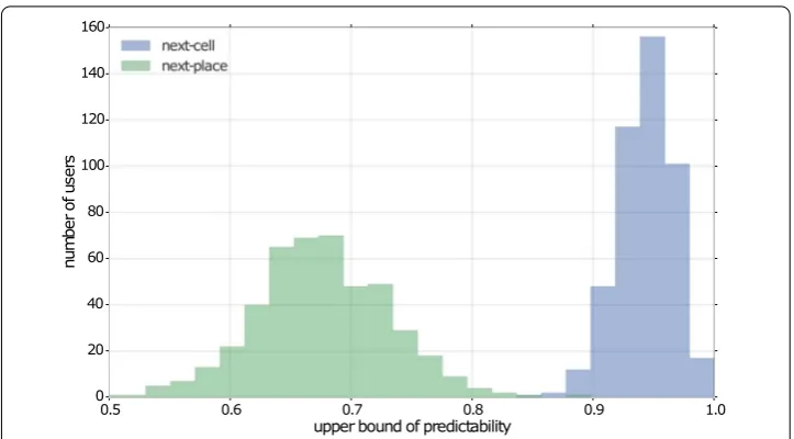
In this formulation, the prediction problem can be restated as follows: given your past cell sequence up to timet, which cell will you visit at timet+t? Before attempting any prediction, we follow the process suggested in [13] and calculate the theoretical upper limit for the predictability of the sequence of cells. Figure 1 shows how the maximum predictability for the grid cell formulation is peaked at around 0.95.

We now consider different baseline strategies for next grid cell prediction. For each of the strategies, we perform prediction in an online manner, by training the algorithm on the data up to timestept, and predicting cell at timestept+t. We measure the accuracy as number of correct predictions over the number of total predictions.

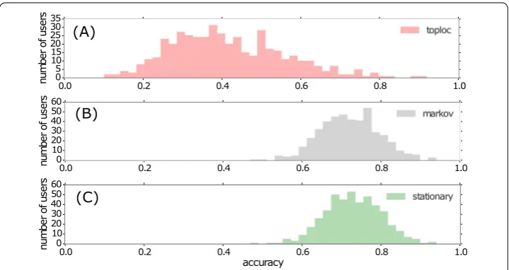
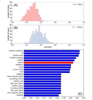
We first consider thetoplocstrategy, where at each timestep we predict the most fre-quent symbol in the history so far (Algorithm 1). Given the highly stationary nature of most human mobility trajectories, we expect this simple strategy to achieve relatively high accuracy. Figure 2(A) shows the distribution of accuracies for all the users. The accuracy of thetoplocis indeed reasonable, peaking at around 0.4.

Figure 1 Upper bound of predictability for all users for the next-cell and next-place formulations.

Algorithm 1Toploc prediction algorithm

1: functiontoploc(locations)

2: C← {}

3: for linlocations do

4: iflnot inCthen

5: C[l]←1

6: else

7: C[l]←C[l] + 1

8: end if

9: end for

10: returni:C[i] = Max(C[:])

11: end function

locations are estimated based on past transitions in the location history. For making a pre-diction, we then consider the transition that has the highest probability among all possible transitions from the current cell. If the current state has never been seen before, then we have no information about the transition probability to other states. In this case we fall back to the toploc strategy and predict the most frequent state. Again we fit the model in an online manner, updating at each step the transition probabilities and then making a prediction for the next timestep. Figure 2(B) shows the distribution of accuracies for all the users. The accuracy of theMarkovmodel is significantly higher than toploc, peaking at around 0.7.

Figure 2 Accuracy of the prediction in the next-cell formulation. (A)The results of the toploc strategy, that predicts the most common location at each step.(B)The accuracy for the Markov chain model.(C)The accuracy for the stationary strategy, that predicts remaining stationary in the previous cell.

Algorithm 2Markov prediction algorithm

1: functionmarkov(locations)

2: m← |unique(locations)|

3: T←0m,m

4: n← |locations|

5: for i= 0 ton– 2 do

6: a←locations[i]

7: b←locations[i+ 1]

8: T[a][b]←T[a][b] + 1

9: end for

10: current←locations[n– 1]

11: ifT[current][:] = 0 then

12: returntoploc(locations)

13: else

14: returni:T[current][i] = Max(T[current][:])

15: end if

16: end function

Algorithm 3Stationary prediction algorithm

1: functionstationary(locations)

2: n← |locations|

3: returnlocations[n– 1]

4: end function

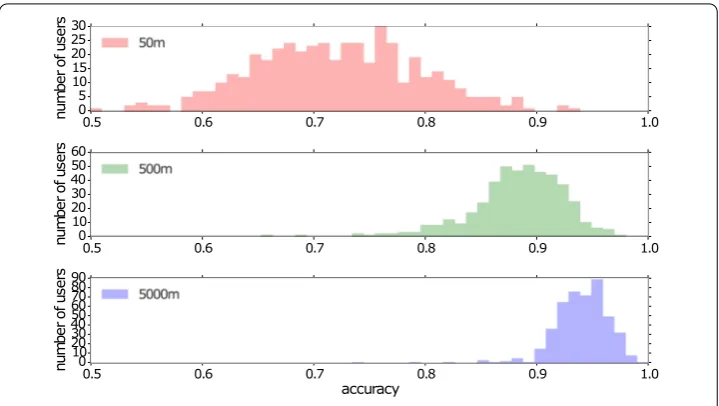
Figure 3 Effect of spatial granularity of the accuracy for the Markov model in the next-cell formulation.Each panel shows the accuracy for a different spatial bin size: 50 m, 500 m and 5000 m. Increasing the size of the spatial bins increases the accuracy prediction.

We now investigate another issue related to the next cellproblem formulation. Intu-itively, we expect that the size of our spatial units will influence the accuracy of predic-tion. Predicting a user’s location with the precision of few meters is intuitively much more difficult that predicting with precision of several kilometers, cf. [18]. In order to exam-ine the effect of spatial resolution, we also consider results for cell sizes of 500 meters and 5000 meters, and apply theMarkovmodel. Figure 3 compares the accuracy for dif-ferent spatial resolutions. As expected the accuracy improves strongly as the spatial size increases.

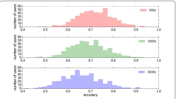
Finally we investigate the effect of temporal resolution within this problem formulation. Our findings above suggest that using a very fine-grained temporal resolution will increase the number of self-transitions, thus driving up the accuracy of the prediction that is mainly able to capture stationarity. We achieve this by discretizing the location at 50 meters cell size, but varying the temporal time binning to 15 minutes, 30 minutes and 60 minutes, and then running theMarkovmodel for each scenario. Figure 4 compares the accuracy for different temporal resolutions. As expected, accuracy is decreased as the time-bins grow larger due fewer self-transitions. We also study the accuracy versus the training size, and we find that the models converge after 50-100 samples (Additional file 1 Figure 6).

3.3 Next-place prediction

Figure 4 Effect of temporal sampling of the accuracy for the Markov model in the next-cell formulation.Each panel shows a different temporal bin resolution: 900 s, 1800 s and 3600 s. Decreasing the temporal resolution in this problem formulation increases the accuracy, since there are more self-transitions.

t1, . . . ,tnare analyzed sequentially in time, and are grouped into a stop whenever they are

within a distance threshold. That is, the distance between position at timetandt+t is less than a thresholdδ= 50 meters, roughly corresponding to the GPS accuracy. If a new location sample is farther away thanδ, then a new stop is created. This produces a sequence of stops, each one with a centroid calculated as the median of the locations co-ordinates, and a duration equal to the time between the last location and the first location sample. In order to filter out the short stops that arise, e.g. during commutes, we consider only stops with duration greater than 15 minutes.

We now group stops into places, where a ‘place’ is a group of spatially proximate stops representing a self-contained area such as a building. Example of places are a ‘home loca-tion’, a ‘work location’ or a restaurant. In order to group the stops, we apply the DBSCAN [38] clustering to the stops in the geographical coordinate space, using the haversine dis-tance. We set as parameter the grouping distance= 50 meters, andmin_pts= 2. This distance threshold is set to produce places of the approximate size of a large building (but our results are robust to reasonable variation of this parameter). The result of the DBSCAN clustering is an assignment of a cluster label to each stop, where the label rep-resents the place that the stop belongs to. Finally, in order avoid artifacts due to missing samples or noise, we merge multiple consecutive stops at the same place into one. The pro-cess described above converts the raw location history into a sequence of stops at places (Additional file 1 Figures 4 and 5).

The prediction task can now be re-formulated as follows: given a sequence of stops up to stepn, can we predict your next place at stepn+ 1? Notice that a key difference from the cell grid formulation is that in this case there are (by definition) no self-transitions; we are interested in the place changes only.

We now apply the two prediction strategiestoplocandMarkovto this new formulation. The two models remain conceptually the same as above, but instead of predicting the grid cell at each time step, they now predict the next place (note that in this formulation we cannot use thestationarystrategy, since - by construction - we are interested in transitions to new places). In this case we also fit each user separately, and we perform the prediction in an online manner. Figure 5(A) and (B) show the accuracy for both models. It is evident that the accuracy for these models (around 0.3 for toploc and 0.4 for Markov) is dramat-ically lower than in thenext-cellformulation, indicating that this problem formulation is a more challenging task.

Another group [39] has independently analyzed the Copenhagen Networks Study data considering similar questions related to predictability; their conclusions are similar to ours. Our work, however, significantly differs in the sense that we study additional factors that influence predictability, in particular the role of contextual features, and the explo-ration of new locations.

3.4 Importance of contextual features

We have investigated how the details of the problem formulation impact the reported accuracy for location prediction tasks. We now focus on next-place prediction and study the influence of different contextual features on performance in the prediction task. We formalize the problem as follows: At each step, we aim to compute the most probable next location given the current location, as well as other context variables, such as time of the day or call activity. In other words we wish to computeP(Lˆ|c1,c2,c3, . . . ,cn), whereLˆis the

next location, andc1,c2,cnare the variables representing different contexts.

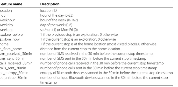
For this purpose we use a logistic regression model, and study how contextual features impact our ability to predict an individual’s next place. The goal of this model is not to sug-gest a new state-of-the-art method, but rather to evaluate the importance of various con-textual features. Specifically, we consider the current location, the time metadata (hour of the day, day of the week, hour of the week, weekend), a ‘home’ binary indication, distance from home, call and SMS activity, and Bluetooth proximity. Table 1 provides a summary of the features.

The logistic regression model defines a linear function of the predictor variables, and then estimates the probability of the target variableLˆusing the logit transformation:

φ(c1,c2, . . . ,cn) =β0+β1c1+β2c2+· · ·+βncn,

P(Lˆ|c1,c2, . . . ,cn) =

1 1 +e–φ.

As there is no closed form solution for setting the weights, the fit is done by numerical optimization with objective of maximizing classification accuracy.

We model each user separately since our goal is to understand next-place prediction at the individual level. We perform online predictions where we fit the data up to stepn, and then predict the next location at stepn+ 1 using a multinomial logistic regression model; classes are simply the set of all possible places visited so far. We fit one model for each individual feature separately, then models combining location and time metadata (hour of the day, hour of the week and day of the week) and then a model with all the features. Models are fit using L2 regularization in order to reduce the number of features. Figure 5(C) displays the accuracy for each of the models, averaged by user.

Table 1 Description of the features used for the logistic regression models

Feature name Description

location location ID

hour hour of the day (0-23)

weekhour hour of the week (0-167)

weekday day of the week (0-6)

weekend sat/sun (1) or Mon-Fri (0)

explore_before 1 if the previous stop is an exploration, 0 otherwise explore_now 1 if the current stop is an exploration, 0 otherwise

home 1 if the current stop is at the home location (most visited place), 0 otherwise d_from_home distance from the current stop to the home location

sms_received_30min number of SMS received in the 30 min before the current stop timestamp sms_sent_30min number of SMS sent in the 30 min before the current stop timestamp

calls_received_30min number of phone calls received in the 30 min before the current stop timestamp calls_sent_30min number of phone calls sent in the 30 min before the current stop timestamp bt_entropy_30min entropy of Bluetooth devices scanned in the 30 min before the current stop timestamp bt_unique_30min number of unique Bluetooth devices scanned in the 30 min before the current stop

The Markov chain model baseline is highlighted in red. Using the current location and time features, the logistic regression model outperforms the Markov chain based model. Even using the current location only (which is conceptually very similar to a Markov chain model), the logistic regression shows stronger performance, likely due to the explicit op-timization of the model. It is interesting that other context variable such as call and SMS data have little predictive power in this model formulation. The most complex model that considers all features is practically identical in performance to the model using only cur-rent location and hour of the week.

The logistic regression model does improve the accuracy over the Markov model, but the absolute value of accuracy still remains low (below 45%). Although the current model could be further fine-tuned, our goal here is not to produce a state-of-the-art prediction model, but instead to investigate the limitations and sources of predictability in human mobility. We also verify the model convergence by studying the accuracy versus the train-ing size, and we find that also in this case the accuracy converges after 50-100 samples (Additional file 1 Figure 6). The logistic regression model shows that (in the current prob-lem formulation) the contextual variables add very little additional predictive power. The next sections will therefore be focused on understanding the factors limiting the predic-tion accuracy.

3.5 Understanding the set of location states

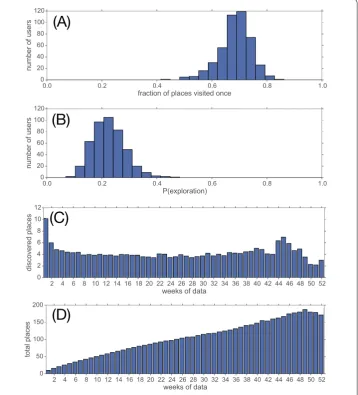
It is well known that the majority of individuals tend to spend most of the times at very few places such as home and work, and only sporadically visit other places. This phenomenon has been described using concepts such as preferential return [40], heavy-tailed stay times and return rate based on the number of visits [41]. For the location prediction tasks, the consequence is that the target classes are unbalanced, which implies that most records be-long to very few classes and most classes are represented by only few records. To illustrate this problem, we consider the extreme case of places visited only once. Figure 6(A) shows that surprisingly this fraction is quite large (0.7). This fact is, in large part, the central reason behind the difficulty of the prediction task.

As we shall see below, another central challenge is not just that our population visits a large number of different places, but also that many new places are discovered over time. We consider a stop at a place as an ‘exploration’ if this place has not been seen in the location history so far for a given user. In other words, this place is being visited for the first time by the user. To express this formally, we consider the sequence of stopss1,s2,s3, . . . ,sn

for each user. We consider a stop si asreturn (Y= 0) if si has been seen before in the

location history, that is there exists a stopsj=sifor 1≤j<i. Otherwise we consider stop

sianexploration(Y= 1), that is the placesiis visited for the first time at stepi. For example

given a location sequence A B A C B C, the target variable exploration would have values 1 1 0 1 0 0.

We can now estimate the probability of exploration as fraction of explorations over the number of stops. To our surprise, this probability is large: between 0.2 and 0.25 (Fig-ure 6(B)). This implies that most users discover a new place every 4 or 5 stops.

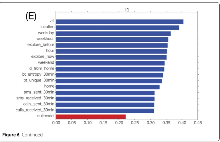
Figure 6 (A)For each user we measure the fraction of places visited only once. This fraction is surprisingly large, as for each user on average 70% of the places were visited only once.(B)The probability of exploration estimated as fraction of explorations over the number of stops per user. This probability is quite large, meaning that on average users discover a new place every 4 or 5 stops.(C)Number of new visited (explored) places for each week, average by user. Surprisingly, the number of explored places does not decrease over time, but remains around 4. This highlights the highly exploring behavior of our population.(D)Cumulated number of new visited (explored) places for each week, average by user. As consequence of the large amount of exploration, the number of possible places to visit increases steadily over time, reaching on average almost 200 in one year.(E)Exploration prediction:f1score for all models.

Figure 6Continued

These facts suggest that the exploration phenomenon is a key reason for the relatively low accuracy of mobility prediction tasks at high spatial resolution. Given the importance of exploration, we now introduce a new task in mobility prediction:exploration prediction.

3.6 Exploration prediction

The exploration prediction task can be phrased as follows: given a user’s location history up to stepn, will the stop at stepn+ 1 be an exploration or a return?

The first question is: how do we express a useful baseline model for the exploration prediction task? Surprisingly, most literature on human mobility prediction has focused on next location prediction, but has overlooked the exploration prediction problem. Thus, to the best of our knowledge no suitable solution has been proposed for this task. We therefore suggest, as a reasonable baseline, random guessing with probability equal to our prior knowledge of the fraction of explorations:P(exploration)≈0.2.

For our main model we use - as before - the logistic regression model with the features used for the next place prediction model. We add two additional features:explore_nowand explore_before, which capture if the current stop or the previous stops were explorations, respectively. The intuition for these is that multiple explorations may occur in a row, and therefore the current exploration may increase the likelihood for an exploration at the next stop.

As before, we fit each individual separately, and we perform an online prediction, that fits based on the data up to stepn, and predicts exploration at stepn+ 1. We fit one logistic regression model for each of the single features, and a more complex model with all the features at once.

predicted explorations) and recall (the fraction of correctly predicted explorations over all true explorations). Figure 6(E) shows the results of the exploration prediction.

As expected, the model with the most complete set of features outperforms the oth-ers. Among the single feature models, perhaps not surprisingly, the current location fea-ture has the best performance. This finding can be explained by the role of some places as ‘gateways’ for exploration such as public transport hubs (e.g. a central train station). The individual features that perform also well are the time-related ones, in agreement with the intuition that exploration tends to happen to at specific times of the day or week. Theexplore_nowandexplore_beforealso perform well, suggesting an element of burstiness in the exploratory behavior. If we consider our best performing model, we find that it has average precision of 0.3 and recall of 0.65. Overall the performance of this model is far from perfect, showing that the exploration prediction problem is a challenging one.

4 Discussion

We first showed that when interpreting reported results of predictive performance, there are a number of factors to take into consideration. Central among these is the problem formulation itself. This is simply because predicting the next time-bin is a very different (and much easier) task than predicting the next transition. We showed that the most chal-lenging problem is the next-place prediction, which is arguably the most useful task for practical applications such as travel recommendations. Another issue to be taken into ac-count is the spatial resolution of the prediction, here we show how more coarse spatial precision results in an easier task. Similarly the time resolution also has an effect on the predictive power. We suggest that the factors described in this paper should be taken in consideration as context when comparing results from prediction models.

Other than the factors discussed above, we believe that one further reason for perfor-mance differences could be the demographics of the dataset. The data set under study arises from students that have no single workplace but tend to change multiple classes per week, even multiple times per day. Moreover a younger population may have a more irregular schedule and more exploratory behavior. Certainly more work is needed to un-derstand the connection between demographics and predictability. For future research, we suggest considering demographic factors when trying to characterize human mobility, as it has been done, for example, by linking changes in mobility patterns with unemploy-ment status [42].

In this sense, we raise the question on whether the simple location history is enough for successful next-place prediction. As we have discussed, there are strong regularities both in the sequence of visits, and in the daily and weekly temporal patterns of visitation. How-ever, there are a lot of ‘exceptions to the rules’, where schedules change, plans are canceled, and people run late. We speculate that other channels such as email, social media, calen-dar, class schedule may be needed for achieving a satisfying accuracy in the prediction task.

Additional material

Additional file 1: Supplementary Information.(pdf )

Funding

This work is funded in part by the High Resolution Networks project (The Villum Foundation), as well as Social Fabric (University of Copenhagen). The funders had no role in study design, data collection and analysis, decision to publish, or preparation of the manuscript. There was no additional external funding received for this study.

Availability of data and materials

Data is from the Copenhagen Networks study

(http://journals.plos.org/plosone/article?id=10.1371/journal.pone.0095978). Due to privacy consideration regarding subjects in our dataset, including European Union regulations and Danish Data Protection Agency rules, we cannot make our data publicly available. The data contains high spatio-temporal resolution location traces from which is easy to reconstruct personal mobility patterns and infer sensitive personal information.

We understand and appreciate the need for transparency in research and are ready to make the data available to researchers who meet the criteria for access to confidential data, sign a confidentiality agreement, and agree to work under our supervision in Copenhagen. Please direct your queries to Sune Lehmann, the Principal Investigator of the study, at sljo@dtu.dk.

Ethics approval and consent to participate

Data collection was approved by the Danish Data Protection Agency, and written informed consent has been obtained for all study participants.

Competing interests

The authors declare that they have no competing interests.

Consent for publication

Not applicable.

Authors’ contributions

Designed the study: AC SL MG. Analyzed the data: AC. Wrote the paper: AC SL MG. All authors read and approved the final manuscript.

Author details

1_{DTU Compute, Technical University of Denmark, Richard Petersens Plads Building 324, Kgs. Lyngby, Denmark.}2_{The Niels}

Bohr Institute, University of Copenhagen, Blegdamsvej 17, Copenhagen, 2100, Denmark.3_{Department of Civil and}

Environmental Engineering and Engineering Systems, Massachusetts Institute of Technology, 77 Massachusetts Avenue, 1-290, Cambridge, 02139, United States.4_{Department of City and Regional Planning, UC Berkeley, 406 Wurster Hall,}

Berkeley, 94720, United States.5_{Lawrence Berkeley National Laboratory, Cyclotron Road, Berkeley, 94720, United States.}

Publisher’s Note

Springer Nature remains neutral with regard to jurisdictional claims in published maps and institutional affiliations.

Received: 3 August 2017 Accepted: 26 December 2017 References

1. Lane ND, Mohammod M, Lin M, Yang X, Lu H, Ali S, Doryab A, Berke E, Choudhury T, Campbell A (2011) Bewell: a smartphone application to monitor, model and promote wellbeing. In: 5th international ICST conference on pervasive computing technologies for healthcare, pp 23-26

2. Quercia D, Lathia N, Calabrese F, Di Lorenzo G, Crowcroft J (2010) Recommending social events from mobile phone location data. In: Data mining (ICDM), 2010 IEEE 10th international conference on. IEEE Comput. Soc., Los Alamitos, pp 971-976

4. Lu X, Bengtsson L, Holme P (2012) Predictability of population displacement after the 2010 Haiti earthquake. Proc Natl Acad Sci 109(29):11576-11581

5. Çolak S, Lima A, González MC (2016) Understanding congested travel in urban areas. Nat Commun 7

6. Eagle N, Pentland A (2006) Reality mining: sensing complex social systems. Pers Ubiquitous Comput 10(4):255-268 7. Liao L, Patterson DJ, Fox D, Kautz H (2007) Learning and inferring transportation routines. Artif Intell 171(5):311-331 8. Zheng Y, Zhou X (2011) Computing with spatial trajectories. Springer, Berlin

9. Arentze T, Timmermans HA (2000) A learning based transportation oriented simulation system. Eirass Eindhoven 10. Balmer M, Meister K, Rieser M, Nagel K, Axhausen KW, Axhausen KW, Axhausen KW (2008) Agent-based Simulation of

Travel Demand: Structure and Computational Performance of MATSim-t, ETH, Eidgenössische Technische Hochschule Zürich, IVT Institut für Verkehrsplanung und Transportsysteme

11. Goodchild MF (2007) Citizens as sensors: the world of volunteered geography. GeoJournal 69(4):211-221 12. Batty M (2013) The new science of cities. MIT Press, Cambridge

13. Song C, Qu Z, Blumm N, Barabási A-L (2010) Limits of predictability in human mobility. Science 327(5968):1018-1021 14. Simini F, González MC, Maritan A, Barabási A-L (2012) A universal model for mobility and migration patterns. Nature

484(7392):96-100

15. Schneider CM, Rudloff C, Bauer D, González MC (2013) Daily travel behavior: lessons from a week-long survey for the extraction of human mobility motifs related information. In: Proceedings of the 2nd ACM SIGKDD international workshop on urban computing. ACM, New York, p 3

16. Lin M, Hsu W-J, Lee ZQ (2012) Predictability of individuals’ mobility with high-resolution positioning data. In: Proceedings of the 2012 ACM conference on ubiquitous computing. ACM, New York, pp 381-390

17. Smith G, Wieser R, Goulding J, Barrack D (2014) A refined limit on the predictability of human mobility. In: Pervasive computing and communications (PerCom), 2014 IEEE international conference on. IEEE, Hungary, pp 88-94 18. Lu X, Wetter E, Bharti N, Tatem AJ, Bengtsson L (2013) Approaching the limit of predictability in human mobility.

Scientific Reports 3

19. Song L, Kotz D, Jain R, He X (2006) Evaluating next-cell predictors with extensive wi-fi mobility data. IEEE Trans Mob Comput 5(12):1633-1649

20. Krumme C, Llorente A, Cebrian M, Pentland A (2013) The predictability of consumer visitation patterns. Sci Rep 3:1645

21. Bapierre H, Groh G, Theiner S (2011) A variable order markov model approach for mobility prediction. Pervasive Computing, 8-16

22. Zheng Y, Xie X, Ma W-Y (2010) Geolife: A collaborative social networking service among user, location and trajectory. IEEE Data Eng Bull 33(2):32-39

23. Gao H, Tang J, Liu H (2012) Mobile location prediction in spatio-temporal context. In: Nokia mobile data challenge workshop, vol 41. p 44

24. Laurila JK, Gatica-Perez D, Aad I, Bornet O, Do T-M-T, Dousse O, Eberle J, Miettinen M et al (2012) The mobile data challenge: big data for mobile computing research. In: Pervasive computing

25. Do TMT, Gatica-Perez D (2012) Contextual conditional models for smartphone-based human mobility prediction. In: Proceedings of the 2012 ACM conference on ubiquitous computing. ACM, New York, pp 163-172

26. Do TMT, Dousse O, Miettinen M, Gatica-Perez D (2015) A probabilistic kernel method for human mobility prediction with smartphones. Pervasive Mob Comput 20:13-28

27. Scellato S, Musolesi M, Mascolo C, Latora V, Campbell AT (2011) Nextplace: A spatio-temporal prediction framework for pervasive systems. In: Pervasive computing. Springer, Berlin, pp 152-169

28. Sadilek A, Krumm J (2012) Far out: predicting long-term human mobility. In: Proceeding AAAI’12 proceedings of the twenty-sixth AAAI conference on artificial intelligence

29. Cho E, Myers SA, Leskovec J (2011) Friendship and mobility: user movement in location-based social networks. In: Proceedings of the 17th ACM SIGKDD international conference on knowledge discovery and data mining. ACM, New York, pp 1082-1090

30. Sadilek A, Kautz H, Bigham JP (2012) Finding your friends and following them to where you are. In: Proceedings of the fifth ACM international conference on Web search and Data mining. ACM, New York, pp 723-732

31. Stopczynski A, Sekara V, Sapiezynski P, Cuttone A, Madsen MM, Larsen JE, Lehmann S (2014) Measuring large-scale social networks with high resolution. PLoS ONE 9(4):95978

32. Kang JH, Welbourne W, Stewart B, Borriello G (2004) Extracting places from traces of locations. In: Proceedings of the 2nd ACM international workshop on wireless mobile applications and services on WLAN hotspots. ACM, New York, pp 110-118

33. Zheng VW, Zheng Y, Xie X, Yang Q (2010) Collaborative location and activity recommendations with gps history data. In: Proceedings of the 19th international conference on World Wide Web. ACM, New York, pp 1029-1038

34. Thierry B, Chaix B, Kestens Y (2013) Detecting activity locations from raw gps data: a novel kernel-based algorithm. Int J Health Geogr 12(1):1

35. Zhou C, Frankowski D, Ludford P, Shekhar S, Terveen L (2007) Discovering personally meaningful places: an interactive clustering approach. ACM Trans Inf Syst 25(3):12

36. Zheng Y, Zhang L, Xie X, Ma W-Y (2009) Mining interesting locations and travel sequences from gps trajectories. In: Proceedings of the 18th international conference on World Wide Web. ACM, New York, pp 791-800

37. Montoliu R, Gatica-Perez D (2010) Discovering human places of interest from multimodal mobile phone data. In: Proceedings of the 9th international conference on mobile and ubiquitous multimedia. ACM, New York, p 12 38. Ester M, Kriegel H-P, Sander J, Xu X (1996) A density-based algorithm for discovering clusters in large spatial

databases with noise. AAAI Press, Menlo Park, pp 226-231

39. Ikanovic EL, Mollgaard A (2017) An alternative approach to the limits of predictability in human mobility. EPJ Data Sci 6(1):12

40. Song C, Koren T, Wang P, Barabási A-L (2010) Modelling the scaling properties of human mobility. Nat Phys 6(10):818-823

42. Toole JL, Lin Y-R, Muehlegger E, Shoag D, González MC, Lazer D (2015) Tracking employment shocks using mobile phone data. J R Soc Interface 12(107):20150185