Examining characteristics of predictive
models with imbalanced big data
Tawfiq Hasanin
1, Taghi M. Khoshgoftaar
1, Joffrey L. Leevy
1*and Naeem Seliya
2Introduction
A generally established set of data-related properties is used to characterize and define big data, including volume, variety, velocity, variability, value, and complexity [1]. The volume of data is likely the best-known characteristic of big data, especially if datasets exceed 1 million instances. Variety is associated with big data because with such data analysis scenarios, one may have to collectively handle structured, unstructured, and semi-structured data. Velocity reflects the high speed with which data is being gener-ated, collected, and refreshed in a big data scenario, in addition to issues of immediate
Abstract
High class imbalance between majority and minority classes in datasets can skew the performance of Machine Learning algorithms and bias predictions in favor of the major-ity (negative) class. This bias, for cases where the minormajor-ity (positive) class is of greater interest and the occurrence of false negatives is costlier than false positives, may result in adverse consequences. Our paper presents two case studies, each utilizing a unique, combined approach of Random Undersampling and Feature Selection to investigate the effect of class imbalance on big data analytics. Random Undersampling is used to gen-erate six class distributions ranging from balanced to modgen-erately imbalanced, and Fea-ture Importance is used as our Feature Selection method. Classification performance was reported for the Random Forest, Gradient-Boosted Trees, and Logistic Regression learners, as implemented within the Apache Spark framework. The first case study utilized a training dataset and a test dataset from the ECBDL’14 bioinformatics competition. The training and test datasets contain about 32 million instances and 2.9 million instances, respectively. For the first case study, Gradient-Boosted Trees obtained the best results, with either a features-set of 60 or the full set, and a negative-to-positive ratio of either 45:55 or 40:60. The second case study, unlike the first, included training data from one source (POST dataset) and test data from a separate source (Slowloris dataset), where POST and Slowloris are two types of Denial of Service attacks. The POST dataset con-tains about 1.7 million instances, while the Slowloris dataset concon-tains about 0.2 million instances. For the second case study, Logistic Regression obtained the best results, with a features-set of 5 and any of the following negative-to-positive ratios: 40:60, 45:55, 50:50, 65:35, and 75:25. We conclude that combining Feature Selection with Random Undersampling improves the classification performance of learners with imbalanced big data from different application domains.
Keywords: Big data, Feature Importance, Feature Selection, Class Imbalance, Machine Learning, Random Undersampling, ECBDL’14, Slowloris, POST
Open Access
© The Author(s) 2019. This article is distributed under the terms of the Creative Commons Attribution 4.0 International License (http://creat iveco mmons .org/licen ses/by/4.0/), which permits unrestricted use, distribution, and reproduction in any medium, provided you give appropriate credit to the original author(s) and the source, provide a link to the Creative Commons license, and indicate if changes were made.
RESEARCH
*Correspondence: [email protected] 1 Florida Atlantic University, 777 Glades Road, Boca Raton, FL 33431, USA
data storage of fast incoming data. The variability aspect of big data reflects issues embedded in this data, such as anomalies and data dimension inconsistencies due to disparate data sources and types. The value characteristics of big data is often seen as the most important attribute because the results of big data analytics are expected to add/increase business value from the data. As briefly stated for the different V’s, the complexity aspect of big data is relatively obvious, and may include issues such as data transformation, relationship of data from different sources, veracity and possible volatility of the collected data. Traditional methods used for mining and analyzing data that do not consider big data are generally unable to handle the various com-plexities associated with big data.
The minimum number of instances in a dataset that defines big data has not been established in the literature. As an example, in [2] that number was set as 100,000 instances. However, in our current work, we set that number as 1,000,000 instances [3, 4]. Globally, the increasing dependence on big data applications neces-sitates the development of efficient techniques for performing knowledge extraction on this type of data. While it is true that class imbalance affects both big and non-big data, the adverse effects are usually more pronounced in the former. Extreme degrees of class imbalance may exist within big data [5] due to massive over-representation of the negative (larger) class within datasets.
Any dataset containing majority and minority classes, e.g., normal traffic and mali-cious traffic flowing through a computer network, can be viewed as class-imbalanced. There are various degrees of class imbalance, ranging from slightly imbalanced to rar-ity. Rarity in a dataset involves comparatively inconsequential numbers of positive instances [6], e.g., the occurrence of 40 fraudulent transactions within an insurance claims dataset of 1,000,000 normal transactions. Binary classification is frequently utilized to focus on class imbalance because many non-binary (i.e., multi-class) clas-sification problems can be addressed by transforming the given data into multiple binary classification tasks. The minority (positive) class, which makes up a smaller portion of the dataset, is usually the class of interest in real-world problems [2]. This is in contrast to the majority (negative) class, which makes up the larger portion of the dataset.
One approach for addressing class imbalance involves the generation of new datasets which have different class distributions than that of the original dataset. To accomplish this, data scientists use data sampling, of which the main categories are undersampling and oversampling. Undersampling removes instances from the majority class, and if done randomly, the technique is known as Random Undersampling (RUS) [11]. Over-sampling adds instances to the minority class, and if done randomly, the technique is known as Random Oversampling (ROS) [11]. Synthetic Minority Over-sampling TEch-nique (SMOTE) [12] is a method of oversampling that creates artificially new instances between minority instances lying relatively close to each other. RUS has been recom-mended over ROS and SMOTE because this undersampling technique imposes a lower computational burden and results in a faster training time, which is beneficial to data analytics [13]. Another approach uses Feature Selection (FS) to address class imbalance. The technique selects the most influential features that can provide information on dis-crimination between classes, given the dataset suffers from class imbalance [14, 15]. This leads to a reduction of the adverse effects of class imbalance on classification perfor-mance [16–18].
In our paper, we present two case studies, each utilizing a combined approach of RUS and FS to investigate the effect of class imbalance on big data analytics. We used: (1) RUS to generate six different class distributions ranging from balanced to moderately imbalanced, and (2) Feature Importance (FI) as a method of FS. Classification perfor-mance was reported for the Random Forest (RF), Gradient-Boosted Trees (GBT), and Logistic Regression (LR) learners, as implemented within the Apache Spark framework. This framework, popular for its speed and scalability, performs in-memory data process-ing [2]. The first case study employs a training dataset and a test dataset from the Evolu-tionary Computation for Big Data and Big Learning (ECBDL’14) [19, 20] bioinformatics competition. The training and test datasets both have 631 features, and contain about 32 million instances and 2.9 million instances, respectively. For the first case study, GBT obtained the best results, with either a features-set of 60 or the full set, and a negative-to-positive class ratio of either 45:55 or 40:60. The second case study, unlike the first, includes training data from one source (POST dataset) [21] and test data from a separate source (Slowloris dataset) [22]. POST and Slowloris are two types of Denial of Service (DOS) attacks. The POST dataset contains 13 features and about 1.7 million instances, while the Slowloris dataset contains 11 features and about 0.2 million instances. For the second case study, LR obtained the best results, with a features-set of 5 and any of the following negative-to-positive ratios: 40:60, 45:55, 50:50, 65:35, and 75:25. We conclude that combining FS with RUS improves the classification performance of learners from different application domains.
To the best of our knowledge, our work is unique in investigating the combined approach of using RUS and FS to mitigate the effect that class-imbalanced big data has on data analytics. In addition, we demonstrate the effectiveness and versatility of our approach with case studies involving imbalanced big data from different application domains.
Slowloris datasets; “Methodologies and empirical settings” section describes the differ-ent aspects of the methodology used to develop and implemdiffer-ent our approach, including the big data processing framework, classification algorithms, FS, and performance met-rics; “Approach for case studies experiments” section provides additional information on the case studies, including steps taken to remedy potential issues associated with the data; “Results and discussion” section presents and discusses our empirical results; and
“Conclusion” section concludes our paper with a summary of the work presented and
suggestions for related future work.
Related work
Our search for related literature extended as far back as 2010, with a focus on published works that use FS and RUS to address imbalanced big data. To the best of our knowl-edge, we were unable to find any studies that satisfied all our search parameters. There are several recent studies on the use of joint approaches of RUS and FS [23–25], but our focus on imbalanced big data with the combination of RUS and FS is unique, as explained in “Methodologies and empirical settings” section.
One related study used real-world data for Android malware app detection [26]. The default dataset contained about 425,000 benign and 8500 malicious apps (instances), a majority-to-minority ratio of 50:1. In our view, the study uses large data and not big data. The authors conducted six experiments, two of which are relevant to our research focus in this paper. Classification performance in their study was assessed with the k-nearest neighbor (k-NN) classifier.
The first of the two relevant experiments investigated the effect of feature extraction on classification performance. For feature extraction, the authors used two independent approaches: Drebin [27] and DroidSIFT [28]. The Drebin method reduced an emulated set of 1,000,000 features to 2246. With Drebin, the authors noted there was no change in True Positive Rate ( TPrate ) (98.2%) and a decrease in False Positive Rate ( FPrate ) from 1.5 to 0.1%. The DroidSIFT method reduced an emulated set of 1183 graph-based features to 192. With DroidSIFT, TPrate and FPrate increased from 90.6 and 18.8% to 95.6 and 22.1%, respectively. The second experiment examined the relationship between class imbalance and classifier performance. Starting with a 1:1 class ratio and 8500 instances for both the benign and malicious apps, the authors used undersampling to produce other majority-to-minority ratios, including 5:1, 10:1, 20:1, 50:1 and 100:1. The transition from a ratio of 1:1 to 100:1 resulted in a negligible increase in TPrate and FPrate from 96.1 and 5.7% to 96.2 and 5.8%, respectively. The authors concluded that: (1) FS is beneficial for the k-NN classifier, and (2) k-NN classification performance is affected by high-class imbalance.
benign and 8500 malicious apps (a majority-to-minority ratio of 50:1). The fact that the study is based on large data is not a shortcoming per se, but a similar study on big data would be more valuable to contemporary, machine-learning research. Also, it is worth noting that the paper addresses a set of specific research questions, none of which directly involve proposed techniques for class-imbalance mitigation.
Another related study is based on a proposal to implement SMOTE within a dis-tributed environment via Apache Spark [29]. With regards to small datasets, the researchers in [29] recognized that there is a standard implementation of SMOTE which supports Python, but distributed computing environments for large datasets cannot benefit from this implementation. To address this deficiency, the ECBDL’14 test dataset was split into a new training dataset and test dataset (80:20 split, respec-tively), with both sets having the same class imbalance ratio as the original test set. Performance metrics such as Area Under the Receiver Operating Characteristic Curve (AUC), Geometric Mean (GM), and Recall were then obtained for RF and Distributed RF classifiers.
We calculated True Positive Rate ( TPrate ) ×True Negative Rate ( TNrate ) scores for
the no-sampling, SMOTE, and Distributed SMOTE approaches used in [29]. The pro-posed implementation, Distributed SMOTE, had the highest value of 0.169. Use of the ECBDL’14 test dataset as the only source of big data and a lack of comparison of Distributed SMOTE to other techniques, including RUS, are two limitations of this related work.
The dataset used in a third related study [30] contained about 17,000 positive instances and 9,514,000 negative instances, a majority-to-minority of 560:1. This dataset is arguably the largest collection of de-identified patient records of real-world dermatology visits in the US [31], where positive instances represent melanoma cases and negative ones represent non-melanoma cases. The authors applied RUS to the dataset to produce a 65:35 majority-to-minority class ratio. The dataset was then ran-domly split, 70:30, into a training and test set, respectively, with cross-validation, and sensitivity and specificity across various thresholds, used to select an optimal deci-sion threshold. Results show that for the AUC metric, the RF classifier with a score of 0.790 outperforms the Decision Tree (DT) and LR classifiers in relation to predicting whether a dermatology patient has a high risk of developing melanoma.
One limitation of the work of [30] is the use of only one randomly undersampled ratio, the class distribution of 65:35. Our study uses RUS to produce six class distri-bution ratios. In addition, our study considers the joint application of RUS and FS, whereas this related work only uses RUS.
algorithm outperformed the other Feature Selection models, particularly with regards to the minority class.
We do not consider the work of [32] to be a genuine study of imbalanced big data because of the comparatively small number of instances involved (494,021 connections). Furthermore, results would be more meaningful if the CSFSG algorithm was compared against an established Feature Selection algorithm, such as the FI function of the RF classifier.
Case study datasets
The training and test datasets used in the first case study came from a different applica-tion domain than those used in the second case study. In both cases, the big data was preprocessed to construct the model and a comparatively smaller dataset was used to test the built model. The first case study utilized the ECBDL’14 dataset and a separate test dataset, both provided by the ECBDL’14 competition. In the second case study, the POST dataset was used for training and the Slowloris dataset for testing. The ECBDL’14 training and test datasets are considered high dimensional (631 features for both), while the POST and Slowloris datasets are not (13 and 11 features, respectively). Further details on the respective datasets are provided in the following subsections.
ECBDL’14
The ECBDL’14 dataset is a great addition for Protein Contact Map (CM) predictive ana-lytics. This dataset was initially used to train a predictor for another competition called 9th Community Wide Experiment on the Critical Assessment of Techniques for Protein Structure Prediction (CASP9) [20]. Proteins are chains of amino acid (AA) residues with the ability to fold into distinct shapes and features. Two residues of a chain are said to be in contact if their distance is less than a certain threshold [34, 35]. Experimenting with proteins is rather time-consuming [36]. Hence, Protein Structure Prediction (PSP) aims to predict the 3-dimensional structure of a protein based on its primary sequence.
To generate the ECBDL’14 dataset, a diverse set of 2682 proteins with known struc-ture were collected selectively [37] from the Protein Data Bank (PDB) public reposi-tory. The obtained set was apportioned into training and test sets, with a 90–10% split. Instances were generated for pairs of AAs at least 6 positions apart in the chain. This process resulted in the generation of a large training set and test set, with the former having 31,992,921 instances (31,305,192 negatives and 687,729 positives) and the latter having 2,897,917 instances. For the training dataset, about 2% of the instances are in the minority class. The data generation process collected three main types of information (attributes), for a total of 631 features. For additional details, we refer the reader to [37], which explains all features, in addition to their construction details.
POST and Slowloris
attacker and the server to continue. Communication between the two hosts becomes a drawn-out process as the attacker sends messages that are comparatively very small, tying up server resources. This effect is exacerbated if several POST transmissions are done in parallel. Slowloris, another similar exploit, keeps numerous HTTP connections open for as long as possible [22]. During this attack, only partial requests are sent to a web server, and since these requests are never completed the available pool of connec-tions for legitimate users shrinks to zero.
Data collection for POST and Slowloris was done within a real-world network envi-ronment. An ad hoc Apache web server, which was set up within the campus network of Indian River State College (IRSC), served as a viable target. The Switchblade 4 tool from Open Web Application Security Project (OWASP) and a Slowloris.py attack script [41] were used to generate attack packets for POST and Slowloris, respectively. Attacks were launched from a single host computer in hourly intervals. Attack configuration settings, such as connection intervals and number of parallel connections, were varied but the same PHP form element on the web server was targeted during the attack. The result-ing POST dataset contains 1,697,377 instances (1,694,986 negatives and 2391 positives) and 13 features. About 0.1% of instances are in the minority class. The POST dataset is considered to be severely imbalanced. Severely imbalanced data, also referred to as highly imbalanced data or high-class imbalance, is typically bounded between majority-to-minority class ratios of 100:1 and 10,000:1 [2]. The resulting Slowloris dataset con-tains 201,430 instances (197,175 negatives and 4255 positives) and 11 features. About 2% of instances are in the minority class.
Methodologies and empirical settings
Big data processing framework
Nowadays, when big data is considered, the names of many tools and frameworks sur-face within the same context. Data engineers construct packages with well-designed algorithms that lessen the need for customization by the consumer of ML solutions in big data analytics. Such frameworks and tools play a significant role in providing speed, scalability, and reliability to ML with big data. Our work uses a state-of-the-art ML library, MLlib, provided by Apache Spark [42, 43], hereinafter referred to as Spark in this paper. Spark is one of the largest open source projects for big data processing [44]. When compared to traditional ML, it greatly increases the data processing speed while also being quite scalable.
In addition to Spark, we use the Apache Hadoop [45–47] environment, which consists of many big data tools and technologies, two of which are used in our work: Hadoop Distributed File System (HDFS) [48] and Yet Another Resource Negotiator (YARN) [49]. HDFS is highly fault-tolerant and can be deployed on low-cost hardware. YARN splits up functionality by deploying a global Resource Manager and per-application Applica-tion Master with master/slave nodes. The fundamental characteristic of Hadoop is the partitioning of data across many (thousands) hosts, and the parallel execution of applica-tion computaapplica-tion for the given data.
[50] technology. We kept our data partitions invariant and memory use fixed during the experiments for performance stability. Thus, the number of distributed data partitions and the number of the cluster slave nodes were picked based on the available resources of our High Performance Computing (HPC) cluster.
Classifiers
To provide good coverage of more than one family of ML algorithms, our work utilized three learners: LR, RF, and GBT from the Spark MLlib implementation. Unless other-wise stated, we maintained the settings of the default parameters of these learners.
For both RF and GBT, which share several similar parameter settings, the number of trees generated in the training process was set to 100 [6, 51]. The Cache Node Ids was set to True and the maximum memory in megabytes (MB) was set to 1024 for speeding up the tree-building process. A very important factor to consider is the feature subset strategy, at each tree node split, which defines the number of features to be selected ran-domly at each split. The feature subset strategy was set to the square root of the fea-tures based on Breiman’s suggestion for RF [52]. The sub-sampling Rate Fraction of the training data used for learning each decision tree was set to 1.0 [6, 51]. Maximum Bins was set to the maximum number of categorical features for the datasets involved in this study, which was 2 for both case studies. We used the Gini index for the Information Gain (IG) calculation.
The LR max iteration parameter was set to 100. The Elastic Net Parameter, which is in the range of 0 and 1, corresponds to α and was set to 0, indicating an L2 penalty [6, 51]. For more information about the supported penalties, please refer to [42]. Note that Spark’s LR has impeded standardization implementation which was set to True, deter-mining whether to standardize the training features before fitting the model.
Performance metrics and model evaluation
Many studies with ML algorithms use a variety of performance criteria, with no fixed standard to evaluate the outcome of the trained classifiers. Some metrics, such as accu-racy, may apply a naive 0.50 threshold to decide prediction between the two classes, and this is often impractical since in most real-world problems the target classes are imbal-anced, usually with minority and majority classes.
Our work uses the confusion matrix, which is shown in Table 1 [10], for the binary classification problem, where the class of interest is usually the minority class and the opposite class is the majority class, i.e. Positive and Negative, respectively. A list of appli-cable performance metrics are explained as follows:
• True Positive (TP) are positive instances correctly identified as positive. • True Negative (TN) are negative instances correctly identified as negative.
• False Positive (FP), also known as Type I error, are negative instances incorrectly identified as positive.
• False Negative (FN), also known as Type II error, are positive instances incorrectly identified as negative.
• TNrate , also known as Specificity, is equal to TN/(TN + FP).
• The final performance metric score considered in our work is given by TPrate×TNrate [19].
Determining whether Type I or Type II errors are more serious in ML depends on the nature of the problem. If the cost of a Type II error is much higher than the cost of a Type I error, then aiming toward a favorable Type II error rate is the general goal, but without sacrificing the Type I error rate.
Random undersampling
Four RUS ratios, using the negative:positive class ratio order, were initially obtained: 90:10, 75:25, 65:35, and 50:50. These proportions were carefully selected to provide a good range between perfectly balanced and moderately imbalanced. In order to increase the product of TPrate and TNrate as much as possible, while keeping these two metrics
close to each other to relatively balance the Type I and Type II errors, we used RUS to create other ratios where the positive class has more instances than the negative class [19]. Thus, we added two ratios, 45:55 and 40:60.
It is worth noting that the randomization process in RUS promotes information loss from the given data corpus, which may create difficulties for ML classification perfor-mance. Because a sample of instances is usually a fraction of a larger body of data, the classification outcome could differ every time RUS is performed. Therefore, this ran-domness may result in splits that may be considered fair, favorable, or unlucky to the classifier. Unlucky splits, for instance, may retain noisy instances that degrade the classi-fication performance. Favorable splits, on the other hand, may retain very good or clean instances that cause the classifier to perform well, but potentially overfit the model.
Additionally, some ML algorithms, such as the RF and GBT learners used in our study, have inherent randomness built within their implementation. Moreover, due to the random shuffling of instances that we performed prior to each training process, other algorithms such as LR may output different results when the features and/or order of instances is changed.
One way to reduce some of the potential negative effects of randomness is by using repetitive methods [53]. To embrace randomness during our sampling and model build-ing, we performed several repetitions per built model.
Feature Selection
A key aspect of our study is to determine an optimal number of features that should be selected from an imbalanced dataset of big data, for cases where distribution ratios and ML domain datasets vary.
Table 1 Confusion matrix
Actual class Predicted class
Positive Negative
We selected subsets of features with FI, a function within the RF classifier that estimates the most relevant features. An analysis of FI can indicate which features are the most effective in training the RF model. This method is receiving increased attention in many ML-related fields, such as bioinformatics [54]. In our work, FI was used to engineer the available feature space by dropping features that may be consid-ered irrelevant while building the classification model. Results obtained from the use of the new feature space were then compared with those where no Feature Selection was performed.
At each split in every tree in the RF model, the importance of the relevant feature is computed using IG, which is the difference between the parent node’s impurity and the weighted sum of the two child nodes’ impurities. Node impurities measure how well a tree splits data [55]. The accumulation of IG over all separate trees for a given feature is the FI for that specific feature. FI scores from all trees are normal-ized to values between 0 and 1. The total FI importance vector from all trees is nor-malized as well for each feature [56].
Another factor needing attention is categorical features. These do not fit into an ML regression model equation in their raw form. Additionally, if the categorical fea-tures were indexed, LR assumes that there is a logical order or a value of the indi-ces. Such subsets of categorical features are known as ordinal features. A nominal feature, unlike an ordinal one, is a categorical feature whose instances can take a value that cannot be organized in a logical sequence [7]. In our work, all categorical features (nominal) were transformed into dummy variables using a one-hot encod-ing method [57], allowing conversion of nominal features into numerical values. A drawback of this method is that a new number of features equaling C−1 is
gener-ated from each feature, where C is the number of categories belonging to the specific feature, and consequently, the total feature space increases in size.
Figure 1 visualizes the FI scores (scaled between 0 and 1) generated by our study for both original datasets. The horizontal dashed lines represent the cut-offs for FS. The figure also shows the proportions of nominal, continuous, and one-hot encoded features. Figure 1a shows that the feature with the highest score has a con-tinuous value. The features start to score below 0.04 and 0.004 after the top 60 and 120 features, respectively. In Fig. 1b, the feature with the highest score has a one-hot encoded value. Also, it is noticeable that all the features with continuous values (total of 8) are included in the top 20 selected features. For the POST case, we recog-nized the significance of the features of the POST dataset (explanation provided in
“Approach for case studies experiments” section) and used twice as many FS cut-offs
as in the ECBDL’14 case.
Approach for case studies experiments
Case study 1: ECBDL’14 dataset
Our method for the first case study is sequentially outlined in six steps: (1) Select subsets of features using the FI function of the RF learner; (2) Implement one-hot encoding; (3) Create six different distribution ratios with RUS; (4) Distribute the data-sets; (5) Train with the GBT, RF, and LR learners; and (6) Perform model prediction against a separate test set. We performed FS prior to one-hot encoding of the fea-tures, due to the fact that categorical features in this case study have, on average, four values that are well-spread throughout the relevant attributes. Following this strategy prevents the loss of any valuable information from the categories during the FS stage. We performed FS based on the scores generated by FI, obtaining 60 and 120 features. The full set (referred to as ALL) with no Feature Selection was also included. After one-hot encoding, the available feature space increased to 985.
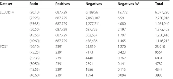
Statistics for the sampled datasets that were generated from the ECBDL’14 dataset are shown in Table 2. The negative percentages in the table were calculated based on the negative (unsampled) total size of 31,305,192 instances.
Case study 2: POST and Slowloris datasets
Our method for the second case study is also sequentially outlined in six steps: (1) Implement one-hot encoding; (2) Select subsets of features using the FI function of the RF learner; (3) Create six different distribution ratios with RUS; (4) Distribute the datasets; (5) Train with the GBT, RF, and LR learners; and (6) Perform model predic-tion against a separate test set (POST is used to build the model, Slowloris is used to test the model). Note that one-hot encoding was performed prior to FS in this second case study, and we provide an explanation for doing this in the following paragraph.
To build an ML model that performs well, it is usually advisable to train the model and test it against data that comes from the same target distribution. However, for the POST case study, we faced the challenge of the training and test data being sourced from different class distributions. Therefore, special attention was given to the origi-nal feature spaces of the training and test sets. For instance, the training set had two features (session flags and attribute) that were not recorded in the test set. To ensure compatibility, those two features were not included in the training process. Moreover, the values of the categorical features in the training set have protocols and flags that were not observed in the test data, and vice versa. This can be problematic for the one-hot encoding method as the dummy variable procedure extends values into new and different features. This issue can be solved in several ways, such as by ignoring the previously unobserved values when transforming the training and/or test sets, thus removing the instances that have these values. However, one reason for not follow-ing this solution is that the unobserved values represent a large number of instances from both the training and test sets. Therefore, to handle such values, we added them as dummy variables to both datasets and filled the entire dummy columns with zeros for each newly generated unobserved feature. After one-hot encoding, the available feature space increased to 72. Since FS occurs after one-hot encoding for this case study, the problem of unobserved features was effectively addressed. We performed FS based on the scores generated by FI, obtaining 5, 10, 20, and 36 features. As in the first case study, the full set of features (referred to as ALL) with no Feature Selection was also included.
Another problem was the processing of missing values. Both training and test data-sets had null values within their categorical features. As Spark ML cannot handle this issue automatically, we explored several options, including: (1) Imputing missing values, (2) Removing the instances that have them, and (3) Taking no action, which means addressing the issue through one-hot encoding. With the third option, a cate-gorical feature containing missing values would have zeroes assigned to all newly gen-erated dummy variables for every instance with missing values. We chose to leave the missing values intact to maintain consistency with the methodology of the first case Table 2 Generated sampled sizes with RUS
a Percentages of negatives are calculated based on the negative (unsampled) total size
Dataset Ratio Positives Negatives Negatives %a Total
ECBDL’14 (90:10) 687,729 6,189,561 19.772 6,877,290 (75:25) 687,729 2,063,187 6.591 2,750,916 (65:35) 687,729 1,277,211 4.080 1,964,940 (50:50) 687,729 687,729 2.197 1,375,458 (45:55) 687,729 562,687 1.797 1,250,416 (40:60) 687,729 458,486 1.465 1,146,215 POST (90:10) 2391 21,519 1.270 23,910
study. Our future studies will explore the challenge of big data analysis with missing values in datasets.
Statistics for the sampled datasets that were generated from the POST dataset are shown in Table 2. The negative percentages in the table were calculated based on the negative (unsampled) total size of 1,694,986 instances.
Results and discussion
The results in Table 3 show the averages of 3 runs per built model in the ECBDL’14 case study and the averages of 10 runs per built model in the POST case study. Only 3 runs were necessary for the ECBDL’14 study because its training dataset is comparatively large and therefore has less statistical variance in scores obtained from the sampled class distributions. All classifier performance results shown were obtained from the product of TPrate and TNrate . We chose these metrics because they are collectively robust enough
for the classification of imbalanced big data, where the product of TPrate and TNrate
should be as high as possible, while keeping them close to each other to relatively bal-ance (as much as possible) the Type I and Type II errors [19]. It is worth noting that using the original (unsampled) training data to build the models yielded TPrate×TNrate
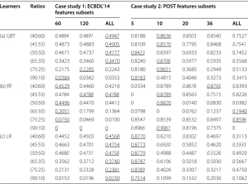
scores of 0, as the models failed to correctly classify any instances from the positive class. Thus, on this account, we did not present the “unsampled” results in our work. For Table 3, the highest value within each column (features-set) of each sub-table is ital-ics and the highest value within each row (class distribution ratio) of each sub-table is underlined. In case study 1, the lowest score of 0 was reported for the 90:10 ratio with RF (all 3 features-set sizes), and the highest score of 0.4947 was reported for the 40:60
Table 3 Empirical results
The highest value within each column (features-set) of each sub-table is in italics and the highest value within each row (class distribution ratio) of each sub-table is underlined
Learners Ratios Case study 1: ECBDL’14
features subsets Case study 2: POST features subsets
60 120 ALL 5 10 20 36 ALL
(a) GBT (40:60) 0.4884 0.4891 0.4947 0.8188 0.8636 0.8503 0.8540 0.7527 (45:55) 0.4873 0.4883 0.4905 0.8109 0.8570 0.7795 0.8468 0.7541 (50:50) 0.4671 0.4737 0.4777 0.8423 0.8397 0.6933 0.8233 0.7452 (65:35) 0.3423 0.3460 0.3470 0.8240 0.8706 0.5977 0.5935 0.5568 (75:25) 0.2175 0.2285 0.2243 0.8180 0.8651 0.3685 0.2949 0.5133 (90:10) 0.0384 0.0382 0.0353 0.8183 0.4815 0.4046 0.3273 0.3415 (b) RF (40:60) 0.4529 0.4460 0.4218 0.0334 0.8789 0.8678 0.8793 0.8393 (45:55) 0.4784 0.4788 0.4788 0 0.8789 0.8563 0.7515 0.8226 (50:50) 0.4496 0.4470 0.4412 0 0.8820 0.0140 0.0830 0.0382 (65:35) 0.2051 0.1799 0.1364 0.0798 0 0.0762 0.1237 0.1940 (75:25) 0.0750 0.0469 0.0190 0.8547 0.8539 0.8532 0.8497 0.8596 (90:10) 0 0 0 0.8966 0.9061 0.8196 0.7375 0 (c) LR (40:60) 0.4452 0.4503 0.4568 0.8770 0.6210 0.8302 0.4697 0.3113
ratio with GBT (features-set of ALL). In case study 2, the lowest score of 0 was reported for the 90:10 ratio with RF (features-set of ALL), and the highest score of 0.9061 was reported for the 90:10 ratio with RF (features-set of 10).
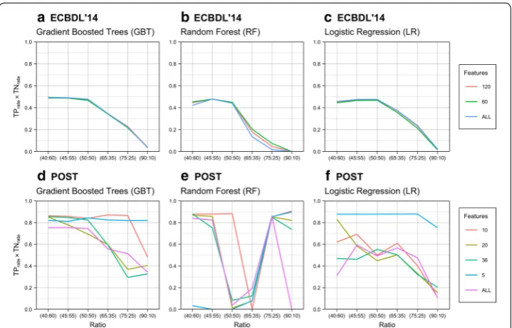
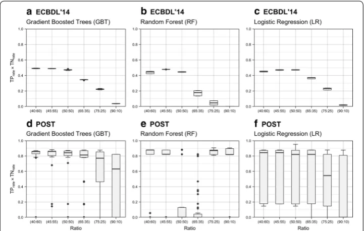
In order to visualize the results shown in Table 3 for the number of selected features used to train the three models for each case study, we included Fig. 2. Figure 2a–c depicts the ECBDL’14 case study and Fig. 2d–f depicts the POST case study. For the ECBDL’14 case, the 3 learners have a similar characteristic curve, with the graphs of GBT and LR closely resembling each other. For the POST case, each learner has a unique set of graphs. The similarity of the curves for the ECBDL’14 case may be because the respec-tive training and test datasets were sourced not only from the same application domain, but also the same available feature space.
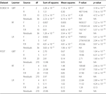
The use of average values for variations of repetitive model building statistically enhances the score results assigned to the models. In addition, to demonstrate statistical significance of the observed experimental results, a hypothesis test is performed using ANOVA [58], and with post hoc analysis via Tukey’s HSD test [59]. ANOVA is a statisti-cal test determining whether the means of one or several independent variables (or fac-tors) are significant. Six rows of two-way ANOVA analysis are shown in Table 4, i.e. three rows for the ECBDL’14 case study and three for the POST case study. The two factors in the table are the number of the selected features (referred to as F in the tables) generated by FI, and sampling class distribution ratios (referred to as R in the tables) generated by RUS. We investigated the intersection of both factors to learn how they affect the respective learner (GBT, RF, LR). If the p-value in the ANOVA table is less than or equal to a certain level (0.05), the associated factor is significant. A 95% ( α=0.05 ) significance level for ANOVA and other statistical tests is the most commonly used value.
A low F-value indicates that the factor has low variability relative to the variability within each group. However, a high F-value is required to reject the null hypothesis, which means the variability of group means is large relative to the variability within each group. Our two-way ANOVA analysis determined that there was a statistically significant difference between groups with only one exception. When classification of the POST dataset was performed with LR, as shown in Table 4, the intersection of the Feature and Ratio factors had no significant effect on the TPrate×TNrate score. How-ever, this intersection proved significant for the GBT and RF learners with the POST dataset, and also for all three learners of the ECBDL’14 dataset.
An ANOVA test may show the results are significant overall; however, not enough information is given on exactly where those differences lie. Therefore, the Tukey’s HSD test compares all possible pairs and finds means of a factor that are significantly different from each other. Differences are grouped by assigning letters (referred to as ‘g’ in the table column headings), with pairs that share the same letter being simi-lar (i.e., no statistically significant difference). Tables 5 and 6, respectively show the Tukey’s HSD tests for both cases in our experimental study. The levels of each fac-tor were averaged and ordered accordingly from the highest to the lowest average. The tables are associated with maximum and minimum values, standard deviation, Table 4 Two-way ANOVA test results
F features subset, R sampling distribution ratio
Dataset Learner Source df Sum of squares Mean squares F-value p-value
ECBDL’14 GBT F 2 2.28 × 10⁻⁴ 1.14 × 10⁻⁴ 18.37 3.18 × 10⁻⁶ R 5 1.51 0.30 48719.46 7.16 × 10−68 F:R 10 2.72 × 10⁻⁴ 2.72 × 10⁻⁵ 4.38 4.72 × 10⁻⁴ Residuals 36 2.23 × 10⁻⁴ 6.19 × 10⁻⁶ NA NA RF F 2 0.007 0.003 9650.57 7.22 × 10−50
R 5 2.12 0.42 1195341.43 6.92 × 10−93 F:R 10 0.01 6.83 × 10⁻⁴ 1927.47 5.37 × 10−46 Residuals 36 1.28 × 10⁻⁵ 3.54 × 10⁻⁷ NA NA LR F 2 0.002 8.07 × 10⁻⁴ 7589.02 5.41 × 10−48
R 5 1.47 0.29 2756163.58 2.04 × 10−99 F:R 10 4.81 × 10⁻⁴ 4.81 × 10⁻⁵ 452.66 9.97 × 10⁻³⁵ Residuals 36 3.83 × 10⁻⁶ 1.06 × 10⁻⁷ NA NA POST GBT F 4 2.70 0.67 13.02 1.04 × 10⁻⁹
R 5 5.17 1.03 19.96 6.31 × 10⁻¹⁷ F:R 20 2.81 0.14 2.71 1.60 × 10⁻⁴ Residuals 270 13.98 0.05 NA NA RF F 4 5.92 1.48 100.68 2.46 × 10−52
R 5 23.38 4.68 317.87 7.03 × 10−111 F:R 20 17.03 0.85 57.90 1.95 × 10−85 Residuals 270 3.97 0.02 NA NA LR F 4 8.11 2.03 22.84 2.89 × 10⁻¹⁶
and quartiles, i.e. first quartile (25th percentile), second quartile (50th percentile or median), and third quartile (75th percentile).
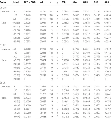
The Tukey’s HSD test revealed that the selection of ALL features and the top 120 features-set from the ECBDL’14 dataset to build the GBT models were statistically insignificant (i.e., yielded similar performances). The test also showed that there is sta-tistical significance between the ALL, 120, and 60 features-set cases for the RF and LR models. Moreover, the percentage differences between the class distributions of 40:60 and 45:55, and 45:55 and 50:50 were noticeably less than the percentage differences between the 90:10 and 75:25, 75:25 and 65:35, and 65:35 and 40:60 distributions. It should be noted that the 75:25 and 65:35 ratios are considered slightly imbalanced, whereas the 90:10 ratio is considered moderately imbalanced. The 90:10 ratio failed to classify any positive class instances with RF. For GBT and LR, this ratio yielded near-zero scores, barely classifying enough positive class instances with accuracy.
Table 5 Tukey HSD test—ECBDL’14 dataset
Factor Level TPR×TNR std r g Min Max Q25 Q50 Q75
(a) GBT
Features ALL 0.3449 0.1741 18 a 0.0343 0.4956 0.2241 0.4111 0.4898 120 0.3440 0.1709 18 a 0.0362 0.4913 0.2283 0.4113 0.4874 60 0.3402 0.1711 18 b 0.0376 0.4910 0.2182 0.4049 0.4862 Ratio (40:60) 0.4908 0.0035 9 a 0.4862 0.4956 0.4878 0.4910 0.4937 (45:55) 0.4887 0.0018 9 a 0.4852 0.4918 0.4878 0.4887 0.4898 (50:50) 0.4728 0.0054 9 b 0.4645 0.4835 0.4691 0.4736 0.4741 (65:35) 0.3451 0.0032 9 c 0.3380 0.3491 0.3437 0.3455 0.3469 (75:25) 0.2234 0.0056 9 d 0.2150 0.2330 0.2196 0.2227 0.2267 (90:10) 0.0373 0.0019 9 e 0.0343 0.0396 0.0362 0.0376 0.0389 (b) RF
Features 60 0.2768 0.1988 18 a 0 0.4787 0.0751 0.3276 0.4529 120 0.2664 0.2043 18 b 0 0.4791 0.0469 0.3132 0.4466 ALL 0.2495 0.2089 18 c 0 0.4792 0.0190 0.2795 0.4412 Ratio (45:55) 0.4787 0.0004 9 a 0.4780 0.4792 0.4785 0.4787 0.4788 (50:50) 0.4459 0.0038 9 b 0.4411 0.4500 0.4413 0.4467 0.4490 (40:60) 0.4402 0.0141 9 c 0.4215 0.4532 0.4222 0.4463 0.4526 (65:35) 0.1738 0.0301 9 d 0.1351 0.2062 0.1375 0.1797 0.2043 (75:25) 0.0470 0.0243 9 e 0.0188 0.0754 0.0191 0.0466 0.0746
(90:10) 0 0 9 f 0 0 0 0 0
(a) LR
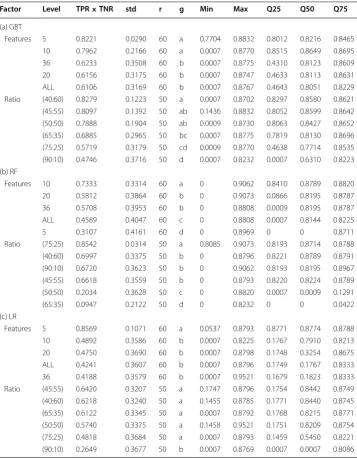
Table 6a–c presents the Tukey’s HSD tests with regards to the POST case. These results show similar, but not exact, behavior with those from the ECBDL’14 case. Inter-estingly, five distribution ratios for LR share the same group letter.
Our ANOVA and Tukey’s HSD test tables show quantitative information and focus on the occurrence of statistical significance, where factors are sufficiently important to be worthy of attention. To provide additional insight into the results, we included Fig. 3. This figure uses box plots to visualize the median (middle quartile or the 50th percen-tile shown as a thick line), two hinges (25th and 75th percenpercen-tiles), two whiskers (also known as error bars), and outlying points. The length of error bars may help reveal the variation of the scores, e.g. a short error bar indicates less variation of scores. Outliers Table 6 Tukey HSD test—POST dataset
Factor Level TPR×TNR std r g Min Max Q25 Q50 Q75
(a) GBT
Features 5 0.8221 0.0290 60 a 0.7704 0.8832 0.8012 0.8216 0.8465 10 0.7962 0.2166 60 a 0.0007 0.8770 0.8515 0.8649 0.8695 36 0.6233 0.3508 60 b 0.0007 0.8775 0.4310 0.8123 0.8609 20 0.6156 0.3175 60 b 0.0007 0.8747 0.4633 0.8113 0.8631 ALL 0.6106 0.3169 60 b 0.0007 0.8767 0.4643 0.8051 0.8229 Ratio (40:60) 0.8279 0.1223 50 a 0.0007 0.8702 0.8297 0.8580 0.8621 (45:55) 0.8097 0.1392 50 ab 0.1436 0.8832 0.8052 0.8599 0.8642 (50:50) 0.7888 0.1904 50 ab 0.0009 0.8730 0.8063 0.8427 0.8652 (65:35) 0.6885 0.2965 50 bc 0.0007 0.8775 0.7819 0.8130 0.8696 (75:25) 0.5719 0.3179 50 cd 0.0009 0.8770 0.4638 0.7714 0.8535 (90:10) 0.4746 0.3716 50 d 0.0007 0.8232 0.0007 0.6310 0.8223 (b) RF
Features 10 0.7333 0.3314 60 a 0 0.9062 0.8410 0.8789 0.8820 20 0.5812 0.3864 60 b 0 0.9073 0.0866 0.8195 0.8787 36 0.5708 0.3953 60 b 0 0.8808 0.0009 0.8195 0.8787 ALL 0.4589 0.4047 60 c 0 0.8808 0.0007 0.8144 0.8225 5 0.3107 0.4161 60 d 0 0.8969 0 0 0.8711 Ratio (75:25) 0.8542 0.0314 50 a 0.8085 0.9073 0.8193 0.8714 0.8788 (40:60) 0.6997 0.3375 50 b 0 0.8796 0.8221 0.8789 0.8791 (90:10) 0.6720 0.3623 50 b 0 0.9062 0.8193 0.8195 0.8967 (45:55) 0.6618 0.3559 50 b 0 0.8793 0.8220 0.8224 0.8789 (50:50) 0.2034 0.3628 50 c 0 0.8820 0.0007 0.0009 0.1291 (65:35) 0.0947 0.2122 50 d 0 0.8232 0 0 0.0422 (c) LR
(represented by dots in the figure) are scores that are numerically distant from the rest of the data, i.e. scores located outside the whiskers.
The top three class distributions for the ECBDL’14 dataset with regards to perfor-mance were consistent for all three learners. These distributions are the 40:60, 45:55, and 50:50 ratios, as shown in Fig. 3a–c. From a performance perspective, there was less consistency for the top three distributions of the POST dataset, as shown in Fig. 3d–f. For instance, Fig. 3d maintained the same top three ranking for GBT when compared with all learners in the ECBDL’14 dataset. However, for Fig. 3e, which corresponds to RF in the POST dataset, the 90:10 and 75:25 ratios were unexpectedly among the top three distributions, and for Fig. 3f, which corresponds to LR in the POST dataset, the 65:35 ratio ranked third. It seems counterintuitive that moderately and slightly imbal-anced ratios of 90:10 and 75:25, respectively, can have higher TPrate×TNrate values than the relevant 45:55 and 50:50 ratios.
For the ECBDL’14 dataset, the GBT selection of 40:60 and 45:55 ratios (group ‘a’) along with ALL and 120 features (group ‘a’) resulted in TPrate×TNrate values of 0.4908 (high-est table value), 0.4887, 0.3449, and 0.3440, respectively, as shown in Table 5. Therefore, the optimal choice for this dataset involves a GBT learner with a combination of one of the ratios from group ‘a’ and one of the features-set sizes from group ‘a’.
With regards to the POST dataset, the LR selection of 40:60, 45:55, 50:50, 65:35, and 75:25 ratios (group ‘a’) along with 5 features (group ‘a’) resulted in TPrate×TNrate values of 0.6218, 0.6420, 0.5740, 0.6122, 0.4818, and 0.8569 (highest table value), respectively,
as shown in Table 6. Therefore, the optimal choice for this dataset involves an LR learner with a combination of one of the ratios from group ‘a’ and a features-set of 5.
Conclusion
This work uniquely investigates the combined approach of using RUS and Feature Selec-tion to mitigate the effect that class imbalance (with varying degrees) has on big data analytics. Through our contribution, we demonstrate the effectiveness and versatility of our method with two case studies involving imbalanced big data from different applica-tion domains. Our results show that Feature Selecapplica-tion and class distribuapplica-tion ratios are important factors.
The best performer in the first case study was the Gradient-Boosted Trees classifier, with either a features-set of 60 or the full set (ALL) of 631 features, and a negative-to-positive ratio of either 45:55 or 40:60. The best performer in the second case study was the Logistic Regression classifier, with a features-set of 5 and any of the follow-ing negative-to-positive ratios: 40:60, 45:55, 50:50, 65:35, and 75:25. It is noteworthy that Logistic Regression, with the features-set of only 5, was a top performer despite the fact that Feature Selection was performed by the Feature Importance function within Random Forest, a different learner. Since the 45:55 and 40:60 class distribu-tions appear in the top selecdistribu-tions for both case studies, we conclude that using RUS to generate class distribution ratios in which the positive class has more instances than the negative class is more likely to be beneficial for big data analytics with imbalanced datasets. This conclusion is particularly applicable for class-imbalanced cases where the test dataset is small relative to the training dataset.
Future work with big data using our combined approach of RUS and Feature Selec-tion will involve addiSelec-tional performance metrics, such as Area Under the Precision-Recall Curve (AUPRC) and AUC, data analysis with missing values in datasets, and the investigation of data from other application domains.
Abbreviations
AA: amino acid; ANOVA: ANalysis Of VAriance; AUC : Area Under the Receiver Operating Characteristic Curve; AUPRC: Area Under the Precision-Recall Curve; CASP9: 9th Community Wide Experiment on the Critical Assessment of Techniques for Protein Structure Prediction; CM: Contact Map; DOS: Denial of Service; DT: Decision Tree; ECBDL’14: Evolutionary Com-putation for Big Data and Big Learning; FI: Feature Importance; FN: False Negative; FP: False Positive; FPrate: False Positive Rate; FS: Feature Selection; GBT: Gradient-Boosted Trees; GM: Geometric Mean; HDFS: Hadoop Distributed File System; HPC: High Performance Computing; HSD: Honestly Significant Difference; HTTP: Hypertext Transfer Protocol; IG: Informa-tion Gain; IRSC: Indian River State College; k-NN: k-nearest neighbor; LR: Logistic Regression; MB: megabytes; ML: Machine Learning; NSF: National Science Foundation; OWASP: Open Web Application Security Project; PDB: Protein Data Bank; PSP: Protein Structure Prediction; RF: Random Forest; ROS: Random Oversampling; RUS: Random Undersampling; SMOTE: Synthetic Minority Over-sampling TEchnique; TN: True Negative; TNrate: True Negative Rate; TP: True Positive; TPrate: True
Positive Rate; YARN: Yet Another Resource Negotiator. Acknowledgements
We would like to thank the reviewers in the Data Mining and Machine Learning Laboratory at Florida Atlantic University. Additionally, we acknowledge partial support by the National Science Foundation (NSF) (CNS-1427536). Opinions, find-ings, conclusions, or recommendations in this paper are the authors’ and do not reflect the views of the NSF. Authors’ contributions
TH carried out the conception and design of the research, performed the implementation and experimentation, performed the evaluation and validation, and drafted the manuscript. TH, JJL, and NS performed the primary literature review for this work. All authors provided feedback to TH and helped shape the research. TH and JJL manuscript the work. TMK introduced this topic to TH, and helped to complete and finalize this work. All authors read and approved the final manuscript.
Availability of data and materials Not applicable.
Ethics approval and consent to participate Not applicable.
Consent for publication Not applicable. Competing interests
The authors declare that they have no competing interests. Author details
1 Florida Atlantic University, 777 Glades Road, Boca Raton, FL 33431, USA. 2 Ohio Northern University, 525 South Main Street, Ada, OH 45810, USA.
Received: 26 May 2019 Accepted: 17 July 2019
References
1. Katal A, Wazid M, Goudar R. Big data: issues, challenges, tools and good practices. In: 2013 sixth international confer-ence on contemporary computing (IC3). 2013. p. 404–9.
2. Leevy JL, Khoshgoftaar TM, Bauder RA, Seliya N. A survey on addressing high-class imbalance in big data. J Big Data. 2018;5(1):42.
3. Soltysik RC, Yarnold PR. Megaoda large sample and big data time trials: separating the chaff. Optimal Data Anal. 2013;2:194–7.
4. Cao M, Chychyla R, Stewart T. Big data analytics in financial statement audits. Account Horizons. 2015;29(2):423–9. 5. Bauder R, Khoshgoftaar T. Medicare fraud detection using random forest with class imbalanced big data. In: 2018
IEEE international conference on information reuse and integration (IRI). 2018. p. 80–7.
6. Bauder RA, Khoshgoftaar TM, Hasanin T. An empirical study on class rarity in big data. In: 2018 17th IEEE interna-tional conference on machine learning and applications (ICMLA). 2018. p. 785–90.
7. Witten IH, Frank E, Hall MA, Pal CJ. Data mining: practical machine learning tools and techniques. Burlington: Mor-gan Kaufmann; 2016.
8. Olden JD, Lawler JJ, Poff NL. Machine learning methods without tears: a primer for ecologists. Quart Rev Biol. 2008;83(2):171–93.
9. Galindo J, Tamayo P. Credit risk assessment using statistical and machine learning: basic methodology and risk modeling applications. Comput Econ. 2000;15(1):107–43.
10. Seliya N, Khoshgoftaar TM, Van Hulse J. A study on the relationships of classifier performance metrics. In: 2009 21st IEEE international conference on tools with artificial intelligence. 2009. p. 59–66.
11. Batista GE, Prati RC, Monard MC. A study of the behavior of several methods for balancing machine learning training data. ACM SIGKDD Explorat Newslett. 2004;6(1):20–9.
12. Chawla NV, Bowyer KW, Hall LO, Kegelmeyer WP. Smote: synthetic minority over-sampling technique. J Artif Intell Res. 2002;16:321–57.
13. Dittman DJ, Khoshgoftaar TM, Wald R, Napolitano A. Comparison of data sampling approaches for imbalanced bioinformatics data. In: The twenty-seventh international FLAIRS conference; 2014.
14. Malhotra R. A systematic review of machine learning techniques for software fault prediction. Appl Soft Comput. 2015;27:504–18.
15. Wang H, Khoshgoftaar TM, Napolitano A. An empirical investigation on wrapper-based feature selection for predict-ing software quality. Int J Softw Eng Knowl Eng. 2015;25(01):93–114.
16. Yin L, Ge Y, Xiao K, Wang X, Quan X. Feature selection for high-dimensional imbalanced data. Neurocomputing. 2013;105:3–11.
17. Mladenic D, Grobelnik M. Feature selection for unbalanced class distribution and naive bayes. ICML. 1999;99:258–67. 18. Zheng Z, Wu X, Srihari R. Feature selection for text categorization on imbalanced data. ACM Sigkdd Expl Newslett.
2004;6(1):80–9.
19. Evolutionary computation for big data and big learning workshop, data mining competition. 2014: self-deployment track. http://crunc her.ico2s .org/bdcom p/.
20. 9th Community Wide Experiment on the Critical Assessment of Techniques for Protein Structure Prediction. http:// predi ction cente r.org/casp9 /.
21. Calvert C, Khoshgoftaar TM, Kemp C, Najafabadi MM. Detecting slow http post dos attacks using netflow features. In: The thirty-second international FLAIRS conference. 2019.
22. Calvert C, Khoshgoftaar TM, Kemp C, Najafabadi MM. Detection of slowloris attacks using netflow traffic. In: 24th ISSAT international conference on reliability and quality in design. 2018. p. 191–6.
23. Wasikowski M, Chen X-W. Combating the small sample class imbalance problem using feature selection. IEEE Trans Knowl Data Eng. 2010;22(10):1388–400.
24. Idris A, Rizwan M, Khan A. Churn prediction in telecom using random forest and pso based data balancing in com-bination with various feature selection strategies. Comput Elect Eng. 2012;38(6):1808–19.
25. Yu H, Ni J, Zhao J. Acosampling: an ant colony optimization-based undersampling method for classifying imbal-anced dna microarray data. Neurocomputing. 2013;101:309–18.
security applications conference. ACSAC 2015. New York: ACM; 2015. p. 81–90. https ://doi.org/10.1145/28180 00.28180 38.
27. Arp D, Spreitzenbarth M, Gascon H, Rieck K, Siemens C. Drebin: effective and explainable detection of android malware in your pocket; 2014.
28. Zhang M, Duan Y, Yin H, Zhao Z. Semantics-aware android malware classification using weighted contextual api dependency graphs. In: Proceedings of the 2014 ACM SIGSAC conference on computer and communications security. New York: ACM; 2014. p. 1105–16.
29. Rastogi AK, Narang N, Siddiqui ZA. Imbalanced big data classification: a distributed implementation of smote. In: Proceedings of the workshop program of the 19th international conference on distributed computing and net-working. New York: ACM; 2018. p. 14.
30. Richter AN, Khoshgoftaar TM. Melanoma risk prediction with structured electronic health records. In: Proceedings of the 2018 ACM international conference on bioinformatics, computational biology, and health informatics. New York: ACM; 2018. p. 194–9.
31. Richter AN, Khoshgoftaar TM. Modernizing analytics for melanoma with a large-scale research dataset. In: 2017 IEEE international conference on information reuse and integration (IRI); 2017. p. 551–8.
32. Bian J, Peng X-G, Wang Y, Zhang H. An efficient cost-sensitive feature selection using chaos genetic algorithm for class imbalance problem. Math Prob Eng. 2016;2016:9.
33. KDD Cup 1999 Data. https ://kdd.ics.uci.edu/datab ases/kddcu p99/kddcu p99.
34. Di Lena P, Nagata K, Baldi P. Deep architectures for protein contact map prediction. Bioinformatics. 2012;28(19):2449–57.
35. Xu Y, Xu D, Liang J. Computational methods for protein structure prediction and modeling volume 1: basic charac-terization. Berlin: Springer; 2007.
36. Stout M, Bacardit J, Hirst JD, Krasnogor N. Prediction of recursive convex hull class assignments for protein residues. Bioinformatics. 2008;24(7):916–23.
37. Triguero I, del Río S, López V, Bacardit J, Benítez JM, Herrera F. Rosefw-rf: the winner algorithm for the ecbdl’14 big data competition: an extremely imbalanced big data bioinformatics problem. Knowl Based Syst. 2015;87:69–79. 38. Liu Y-H, Zhang H-Q, Yang Y-J. A dos attack situation assessment method based on qos. In: Proceedings of 2011
international conference on computer science and network technology. 2011. p. 1041–5.
39. Yevsieieva O, Helalat SM. Analysis of the impact of the slow http dos and ddos attacks on the cloud environment. In: 2017 4th international scientific-practical conference problems of infocommunications. science and technology (PIC S&T). 2017. p. 519–23.
40. Hirakaw T, Ogura K, Bista BB, Takata T. A defense method against distributed slow http dos attack. In: 2016 19th international conference on network-based information systems (NBiS)). 2016. p. 519–23.
41. Slowloris.py. https ://githu b.com/gkbrk /slowl oris. 42. Apache Spark MLlib. https ://spark .apach e.org/mllib /.
43. Zaharia M, Chowdhury M, Franklin MJ, Shenker S, Stoica I. Spark: cluster computing with working sets. HotCloud. 2010;10:10.
44. Meng X, Bradley J, Yuvaz B, Sparks E, Venkataraman S, Liu D, Freeman J, Tsai D, Amde M, Owen S, et al. Mllib: machine learning in apache spark. JMLR. 2016;17(34):1–7.
45. Apache Hadoop. http://hadoo p.apach e.org/. 46. Venner J. Pro Hadoop. New York: Apress; 2009.
47. White T. Hadoop: the definitive guide. Sebastopol: O’Reilly Media, Inc.; 2012.
48. Shvachko K, Kuang H, Radia S, Chansler R. The hadoop distributed file system. In: 2010 IEEE 26th symposium on mass storage systems and technologies (MSST). 2010. p. 1–10.
49. Vavilapalli VK, Murthy AC, Douglas C, Agarwal S, Konar M, Evans R, Graves T, Lowe J, Shah H, Seth S, et al. Apache hadoop yarn: yet another resource negotiator. In: Proceedings of the 4th annual symposium on cloud computing. New York: ACM; 2013. p. 5.
50. Dean J, Ghemawat S. Mapreduce: simplified data processing on large clusters. Commun ACM. 2008;51(1):107–13. 51. Bauder RA, Khoshgoftaar TM, Hasanin T. Data sampling approaches with severely imbalanced big data for medicare
fraud detection. In: 2018 IEEE 30th international conference on tools with artificial intelligence (ICTAI); 2018. p. 137–42.
52. Breiman L. Manual on setting up, using, and understanding random forests v3. 1. 1st ed. Berkeley: Statistics Depart-ment University of California; 2002.
53. Van Hulse J, Khoshgoftaar TM, Napolitano A. An empirical comparison of repetitive undersampling techniques. In: 2009 IEEE international conference on information reuse & integration. 2009. p. 29–34.
54. Strobl C, Boulesteix A-L, Zeileis A, Hothorn T. Bias in random forest variable importance measures: illustrations, sources and a solution. BMC Bioinform. 2007;8(1):25.
55. Raileanu LE, Stoffel K. Theoretical comparison between the gini index and information gain criteria. Ann Math Artif Intell. 2004;41(1):77–93.
56. Friedman J, Hastie T, Tibshirani R. The elements of statistical learning, vol. 1. Springer series in statistics, 2001. 57. Herland M, Khoshgoftaar TM, Bauder RA. Big data fraud detection using multiple medicare data sources. J Big Data.
2018;5(1):29.
58. Iversen GR, Wildt AR, Norpoth H, Norpoth HP. Analysis of variance. 1st ed. Thousand Oaks: Sage; 1987. 59. Tukey JW. Comparing individual means in the analysis of variance. Biometrics. 1949;5:99–114.
Publisher’s Note