Optimizing Transmission Network Expansion Planning With The Mean Of Chaotic Differential Evolution Algorithm

305

Optimizing Transmission Network Expansion

Planning With The Mean Of Chaotic Differential

Evolution Algorithm

Ahmed R.Abdelaziz,Ahmed M.Fathy

Abstract: This paper presents an application of Chaotic differential evolution optimization approach meta-heuristics in solving transmission network expansion planning (TNEP) using an AC model associated with reactive power planning (RPP). The reliability–redundancy of network analysis optimization problems implicate selection of components with multiple choices and redundancy levels that produce maximum benefits, can be subject to the cost, weight, and volume constraints is presented in this paper. Classical mathematical methods have failed in handling convexities and non-smoothness in optimization problems. As an alternative to the classical optimization approaches, the meta-heuristics have attracted lot of attention due to their ability to find an almost global optimal solution in reliability–redundancy optimization problems. Evolutionary algorithms (EAs) – paradigms of evolutionary computation field – are stochastic and robust meta-heuristics useful to solve reliability–redundancy optimization problems. EAs such as genetic algorithm, evolutionary programming, evolution strategies and differential evolution are being used to find global or near global optimal solution. The Differential Evolution Algorithm (DEA) population-based algorithm is an optimal algorithm with powerful global searching capability, but it is usually in low convergence speed and presents bad searching capability in the later evolution stage. A new Chaotic Differential Evolution algorithm (CDE) based on the cat map is recommended which combines DE and chaotic searching algorithm. Simulation results and comparisons show that the chaotic differential evolution algorithm using Cat map is competitive and stable in performance with other optimization approaches and other maps.

Index Terms: Transmission Expansion Network Planning; Differential Evolution (DE); Lozi’s DE; Chaotic DE

————————————————————

1

I

Transmission network expansion planning (TNEP) is a critical issue especially in restructured power systems. Cost-effective transmission expansion planning (TNEP) is a major challenge with regard to electrical power system optimization problem. As electricity consumption grows briskly, TNEP problem is to obtain the optimal expansion plan for an electrical power transmission network [2]. Furthermore, TNEP should specify the newly required transmission facilities that must be added into an existing network to provide adequate system operation and performance over a specified planning horizon, additional transmission lines are required to facilitate alternative paths for power transfer from power plants to load centers. For effective planning, the planner has to determine the exact location, quantity, timing and type of new transmission equipment that is to be installed to satisfy the demand increase, generation additions and increased power flows. For static planning, the planner searches for an appropriate number of new circuits that should be installed into each branch of the transmission system. Based on enhancing component reliability and providing redundancy while considering the trade-off between system performance and resources, a reliability design that aims to obtain an appropriate (or optimal) system-level configuration has long been an important feature in reliability engineering.

TNEP via simplified models such as the transportation model, hybrid model, linear disjunctive model, and DC model, among others, will usually fail to support a solution that can handle real network necessities. On the other hand, with regard to dynamic planning, time-phased or various stages are considered an optimal expansion schedule or strategy is outlined over the completely planning period. A complete and comprehensive model including major aspects of real networks, an AC model, is employed in this research. In fact, transmission planning using an AC model should be associated with reactive power planning (RPP). Without considering reactive sources or VAr-plants, the AC-TNEP problem may have an optimum solution in which only the generators satisfy reactive load demands. Although in case of generator capability of supporting reactive load demands, transferring such an amount of reactive power may reduce the available transfer capability (ATC) that lead to more new transmission lines. Contrariwise, without considering the VAr-plants, load bus voltages may differ from their specified magnitudes, which may not only cause unacceptable power quality but also increase real power losses. Increasing power losses may require more transmission line additions. That is why we propose a concurrent planning approach for the TNEP and RPP problem as a combined methodology. Besides increasing the capacity of transmission lines and power loss reduction due to inclusion of RPP in TNEP, voltage profile enhancement and voltage stability margin improvement can be achieved. The objective function of TNERPP is to determine where, how many and when new equipment such as transmission lines and reactive power sources must be added to the network in order to make its operation viable for a pre-defined planning horizon at minimum cost. Recently, other methods based on artificial intelligence (AI) techniques have been also proposed to solve the TNERPP problem. These AI techniques include genetic algorithms (GAs), simulated annealing (SA), tabu search (TS) and artificial neural networks (ANNs). In 2002, Al Saba and El- Amin applied several types of AI

_____________________________

 Ahmed M.Fathy, Alexandria Higher Institute of Engineering & Technology (AIET), Electronic & Communication Department 2, Alexandria, Egypt, [email protected]

306

techniques, including GAs, TS and ANNs with linear and quadratic programming models, to solve the TNERPP problem. The purpose of the TNERPP was to minimize the investment costs needed to handle the increased load and the additional generation requirements in terms of circuit additions and power losses. Even with the fast convergence of their approach, the obtained solution may not be optimal. Solving the TNERPP problem considering the AC model in one stage is too difficult; particularly in transmission network expansion where the initial topology has isolated areas, the solution might not be easily achieved. In this research the TNERPP problem is managed in three phases: in the first phase, a DC-TNEP is solved to introduce initial solution; in the second phase, by assuming all reactive demands are procured locally, new lines will be added through an AC-TNEP to support power losses. Finally, in the third phase, by removing local reactive sources in the second phase, reactive power planning is handled to find the location and minimum capacities of the VAr-plants needed for feasible system operation. The differential evolution algorithm (DEA) has been applied to optimize a wide range of electrical power system problems such as economic dispatch [1] and, short term scheduling of hydrothermal power system [18], power system planning [6] and optimal reactive power flow [2]. In a number of cases, DEA has proved to be more accurate, reliable and

can provide optimum solutions within acceptable

computational times. Considering such advantages with regard to DEA performance, we propose a novel DEA to solve both the static and multistage TNERPP problem with DC model in this paper. The total investment costs and computational times of different DEA and its modified approaches will be compared with a conventional genetic algorithm (CGA) on the Garver 6-bus system. This paper is organized as follows: in Section 2 TNERPP mathematical modelling of is presented; Section 3 a DE ,CDE solution

algorithm is introduced, while in Section 4 the

implementation of TNERPP proposed methodology is described. In Section 5, a modified 6-Bus Garver system is employed with further analysis through the implementation of the proposed approach, and concluding remarks are presented in Section 6.

2

M

T

A mathematical model for the TNERPP problem can be expressed via Eqs. (1)– (11):

= = (2)

–

Where c and n represent the circuit costs vector and the added lines vector, respectively. N and N0 are diagonal

matrices containing vector n and the existing circuits in the base configuration, respectively. is the cost function of VAr-plants; q is the MVAr size of the VAr-plants vector. u is a binary vector that indicates whether or not to install reactive power sources at load buses. is the investment due to the addition of new circuits to the network, and v1 is

the cost of VAr-plants. is a vector containing the maximum number of circuits that can be added. is the phase angles vector, while and are the existing real and reactive power generation vectors. and are real and reactive power demand vectors; V is the voltage magnitudes vector; , and ̅ are the vectors of maximum real and reactive power generation limits and voltage magnitudes, respectively; , , and are the vectors of minimum real and reactive power generation limits and voltage magnitudes, respectively. In this paper, 105% and 95% of the nominal value are used for the

maximum and minimum voltage magnitude limits,

respectively. , and S are the apparent power flow vectors (MVA) through the branches in both terminals and their limits. The first objective function (1) considers only the expansion costs of transmission lines, while the second objective function (2) considers the minimum costs of the VAr-plants that will be installed. Equations express the limits for real and reactive power for generators are (5) and (6), respectively; for VAr-plants and voltage magnitudes by Eqs. (7) and (8), respectively. Equations present capacity limits (MVA) of the line flows are (9) and (10), while new added circuit constraints are shown in Eq. (11).

The cost of VAr-plants can be defined as follows:

∑

Where k Ωl represents the k

th _{load bus, Ω}

l is the set of all

load buses, and c0k and c1k are the installation costs and

unit costs for a VAr-plant at bus k, respectively. qk is the

MVAr size of a VAr-plant installed at bus k, and uk is a

binary variable that indicates whether or not to install a reactive power source at bus k. The conventional equations of AC power flow considering n is presented in Equation (3) , (4) , the number of circuits (lines and transformers), and q, the size of VAr-plants treated as variables. The elements of vectors and are calculated by Eqs. (13) and (14), respectively:

∑

∑

Where represent _{and buses and is the set}

of all buses, and ij represents the circuit between buses i and j. represents the phase angle difference

307

{

( )

∑( )

}

{

( )

∑ ( )

}

Where , and are the number of buses belong to

conductance, susceptance, and shunt susceptance of the transmission line or transformer ij (if ij is a transformer

_{= 0), respectively, and is the shunt susceptance at}

bus i, while the proposed and codification model represented in table 1 model does not consider the phase shifters. Elements (ij) of vectors _{and of (9) and (10)}

are given by the following relationship:

√

√

1-2 1-4 2-3 3-5 4-5

0 3 1 0 2

Table.1 Codification Proposal

₍

)

Integer variable n, the number of circuits added in branch ij, and the binary variable u, the connection or disconnection of VAr-plants to a load bus, are the most important decision variables where any feasible operation solution of power systems depends on their values. The remaining variables only represent the operating state of a feasible solution in which a feasible investment proposal, defined through specified values of n and u, can include several feasible operation states.

3

DEA

A

Evolutionary Algorithms (EAS), DEA is a population-based stochastic optimizer that starts to explore the search space by sampling at multiple, randomly chosen initial points. It is a kind of float point encoding evolutionary optimization algorithm. AT present, there have been several variants of DEA [1]. One of the most promising schemes, DE/rand/1/bin (DE/best/1/bin) scheme of Storn & Price, is presented in detail. The pseudo code of DEA is given as follows:

Initial Population Generation REPEAT

Mutation Operator Crossover Operator Selection Operator

UNTIL (termination criteria are met)

 DEA operates directly on floating point vectors while CGA relies mainly on binary strings. CGA relies mainly on recombination to explore the search space, while DEA uses a special form of mutation as the dominant operator; DEA is an abstraction of evolution at individual behavioural level, stressing the behavioural link between an individual and its offspring, while CGA maintains the genetic link. There are also a number of significant advantages when using DEA, which were summarised by Price.

 Ability in many cases to find the true global minimum regardless of the initial parameter values; Fast and simple with regard to application and modification; requires few control parameters; Parallel processing nature and fast convergence. Capable of providing multiple solutions in a single run; Effective on integer, discrete and mixed parameter optimisation; Ability to find the optimal solution for a nonlinear constrained optimisation problem with penalty functions.

 Although DEA has many advantages as above

explanation, there are also a number of disadvantages of DEA that are as follows: DEA does not always produce an exact global optimum (premature convergence); DEA may require tremendously high computation time since a large number of complicated fitness evaluations. DEA is a parallel direct search method that employs a population P of size NP, consisted of floating point encoded

individuals or candidate solutions (17).

At every generation G during the optimization process, DEA maintains a population of vectors of candidate solutions to the problem at hand

[ ]

Each candidate solution Xi is a D-dimensional vector,

containing as many integer-valued parameters (18) as the problem decision parameters D

3.1.Generation of Initial Population

The DEA starts with the initializing target population with the population size NP and the dimension

D, which is generated by the following way.

( )

Where i=1, 2… NP, j=1, 2….D, denotes the upper

constraints, and denotes the lower constraints.

3.2.Mutation Operator

For the scheme DE/rand/1/bin, each target vector (i=1, 2… m), a mutant vector is produced by formula (20a),

Where i, r1, r2 {1,2,…, NP } are randomly chosen and

which , , and are selected

308

which has an effect on the difference between the individual

and Basically, scheme DE/best/1/bin works the same

way as DE/rand/1/bin except that it generates the vector according to formula (20b):

Where xbest is the best solution in the current generation.

3.3.Crossover Operator

DE employs the crossover operator to add the diversity of the population. The approach is given below.

{

where i =1,2,…, NP , j =1,2,…, D , CR [0,1] is crossover

constant and rand(i) (1,2,…n) is the randomly selected index. In other words, the trial individual is made up with some of some components of the mutant individual, or at least one of the parameters randomly selected, and some of other parameters of the target individual.

3.4.Selection Operator

To decide whether the trial individual should be a member of the next generation, it is compared to the corresponding xi (t). The selection is based on the survival of

the fitness between the trial individual and the corresponding one such that:

{ ( ) ( )

The DEA optimization process is repeated across generations to improve the fitness of individuals. The overall optimisation process is stopped whenever maximum number of generations is reached.

4

T

C

DEA

A

D

M

The idea of using chaotic systems instead of random processes has been noticed in several fields. The application of chaotic sequences can be a good alternative to maintain the search diversity in stochastic optimization procedures. Due to the ergodicity property, chaos can be used to enrich the searching behaviour and to avoid being trapped into local optimum in optimization problems and we can do this with a several types of maps [5].

4.1.Logistic Map

The algorithm that explores the stochastic serial αj, which

distributes in region [–1, 1] using the improved logistic map. The steps of chaotic differential evolution (CDE) algorithm are summarised as follows[3]:

Step1 Initialisation. Let an evolution generation t = 0. Initialise a population of i = 1, 2, …, NP individuals

(real-valued D dimensional solution vectors) with random values generated according to equation (19).

Step2 Mutation operation according to equation (20)

Step3Crossover operation according to equation (21).

Step4 Selection operation. We have devised an algorithm that explores the global optimal value around and the current best , which tunes the position of the optimal solution using the improved logistic map. Two new individuals, and are calculated with some probability, using the following equations:

( )

_{( )}

Where are distributed in the region [–1, 1] for each j by the following improved logistic map rules

_{( )}

Step4.1. Evaluate objective function value ( ) of each new individuals if ( )< ( ) then go to.

Step5← otherwise ( )> ( ) then go to step 4.2. if

( ) ( ) then go to step 4.4.

Step4.2 Evaluate objective function value ( ) if ( ) ( ) then go to Step 5← otherwise go to step 4.3.

Step4.3 Evaluate objective function value ( ) if ( ) ( ) then go to Step 5 otherwise, go to step 4.4.

Step4.4 go to step5.

Step5 If the stopping criteria is satisfied, then stop; otherwise, let t = t + 1 and go to Step 2.

4.2.Lozi’s Map

The performance of DEA is sensitive to the choice of control parameters. An important issue that needs to be addressed is the value of the parameter F in (20a). The parameter F controls the amplification of the differential variation. To the best of our knowledge, no optimal choice of the scaling parameter F has been suggested in the literature of DEA. This means F is problem-dependent and the user should choose F carefully after some trial and error tests. In this section, a DEA approach using chaotic sequences dynamically adjust the parameters of DEA is proposed. The design of approaches to improve the convergence of DEA optimization is an important issue. A chaotic DEA approach is proposed here based on Lozi’s map. The Lozi’s piecewise liner model [4] is a simplification of the He´non map and it admits strange attractors. The only difference between Lozi’s and He´non’s maps is that the term is replaced by | |. The Lozi’s map is given by:

| |

309

Where k is the iteration number. In this work, the values of y are normalized in the range [0, 1] to each decision variable in N-dimensional space of optimization problem. This transformation is given by

Where [-0.6418, 0.6716] and [ [- 0.6418, 0.6716]. The parameters used in this work are a =1.7 and b = 0.5, these values suggested by [4]. In spite of the prominent merits, sometimes DEA strategy shows the premature convergence and slowing down of convergence as the region of global optimum is approached. It is well established that DEA is particularly sensitive to its control parameters, most notably the mutation factor F(t). In this context, due to the ergodic and dynamic properties of Lozi’s map variables, DEA based on Lozi’s map (LDE) can be useful in mutation factor design for escaping from local optima in optimization problems. The LDE approach is employed to increase the diversity of individuals’ population and prevent the premature convergence of DEA. The LDE approach is a modification of Eq. (20) given by:

Where L(t) is a normalized function w (see Eq. (28)) in the range of [0.1, 0.9] based on the value of y of Lozi’s map. By proposed LDE approach, the probability that the Eq. (20) with F (t) will be utilized is 90% in relation to the Eq. (29). The LDE strategy maintains the diversity of individuals during the evolution.

4.3.Chaotic Cat Map

Chaos is a nonlinear phenomenon that widespread in nature, its movement is ergodicity, randomness and initial sensitive. Chaotic movement could traverse all the status according to its own law. So the optimization search by use of chaotic variable is better than that using random variable. The chaotic searching performs better when in a small searching space and is easy to jump out of the local optimum. Therefore, the chaotic searching is used when DEA fall into the local optimum, to improve the DE performance. It is considered that the DEA has fallen into the local optimum, when the PFV is less than a threshold T. At this time, supposing the best population is [5]:

Generating two random vectors ( )

where The

two-dimensional cat map chaotic sequence and are

calculated by iteration. Supposing

( ) is the chaotic

sequence group to use. Where, N is the limited maximum searching times. Then the chaotic variable is transformed to the optimization variable space in the way of formula (31) and the optimized variable is

( )

It is known from formula (31) that the chaotic variables extended to the circular region where the best population P* is the origin and ri is the radius. The ri is an adjust factor.

When ri is relative large, it is benefit to global searching and

in a low convergence speed, conversely, it is limited in a small region near to the best population which is useful to improve the searching precision.

4.4.The Improved DEA that Based on the Chaotic Searching:

The chaos differential evolution algorithm (CDE) is proposed and its main idea is:

Step.1 The conventional DEA is being executed until it is fall into the local optimum (the PFV is less than a threshold) [5];

Step.2 The chaotic sequence from cat map is calculated and optimized;

Step.3 The random population is instead by the optimized chaotic sequence and the following operations of recombination and selection is executed. The flow chart of CDE is shown as below:

Figure 1. Flow chart of CDE[5]

5

TENRPP

The overall implementation procedure for solving a TNERPP problem using the proposed algorithm is shown in Fig. 2, in which the various steps to find the optimum solution are described as follows:

310

I. Read network data and candidate lines and VAr-plants

that might be installed on the network.

II. Solve the following DC-TNEP, which is a simplified form of the AC model, to find the minimum cost of initial topology for; The TNERPP problem:

| | ̅ ̅ ̅

n is an integer and is unbounded

Where f and are the vectors of total power flow and the corresponding maximum branch flow, respectively. S is the branch-node incidence transposed matrix of the power system. Although the search area is very large, this kind of problem has been developed in many studies [7–9], in which it is solved effectively by introducing some metaheuristics methods and the linearization of the DC model. In the proposed method, n will be replaced by a new topology suggested by CDE in order to convert DC-TNEP to a linear programming problem. Therefore each proposed topology will be treated as an LP problem in order to calculate the fitness function. In fact, after some CDE generation the optimal solution (topology) will be obtained and inserted in the system. After this phase, a completely connected system feasible for the DC model is available, but it could be unfeasible for the AC model.

III. Solve the following mathematical problem, a

constrained AC power flow, to impose the feasibility operation requirements:

̅

is unbounded

This problem considers active and reactive power balances as well as voltage, generators, and apparent power flow constraints. When this problem is satisfied, it seems there is no need to reinforce the transmission network. Else, a power system that may need extra transmission lines or VAr-plants should move to the next step. This problem is solved only once (See Fig. 2).

IV. Solve the following AC-TNEP considering all reactive power demand supplied locally to search for new lines that are necessary for real power loss support:

̅

n is an integer and is unbounded

This problem is a mixed integer nonlinear programming (NLP), but since the search area is quite limited, the solution in this step can be derived after a few repetitions of NLP. As in step II, CDE is employed to handle this NLP problem. In this phase, we identify only the reinforcements needed in transmission lines. Independent of the size of the system, the number of reinforcements in this phase is low, so the processing time is low.

VI. Considering the new transmission lines added in steps II and IV, and the neglected local reactive sources, which were added in the previous section, complete a simple reactive power planning to find the minimum number of VAr-plants that are needed for feasible operation of the power system, and then add the proposed VAr-plants to the network. The problem that is solved in this stage is as follows:

311

This problem is also well addressed in many papers [6–7], while in our proposed methodology this step is solved through a Chaotic DEA. Each topology of VAr-plants allocated by the DEA embedded in the above problem and converted to an NLP problem can be solved with an NLP solver. A solution to the problem becomes feasible by including the transmission lines derived in steps II and IV as well as the VAr plants in step V, and further reinforcement is not needed. The algorithm will therefore stop at this stage. The previous proposal can be easily extended by selecting a reduced set of quality topologies for the DC model at the end of the phase 1, instead of choosing only the best one. Phases 2 and 3 can thus be implemented for each of those topologies, thus increasing the possibility of finding the optimal solution in complex systems.

6

S

,

N

The proposed CDEA procedures were implemented in Matlab R2012b and tested on the electrical transmission networks reported in [7, 8, 9], comparing the results with CGA. In the analyses, the static TNERPP procedure was tested on the following the test systems; 6-bus system originally proposed by Garver [2]. The static TNERPP problem was investigated in two cases that were with and without generation resizing consideration. In case of with generation resizing consideration, the generated MW power at each generator varied from until which the details were explained before. In this experiment, the values of were set to 0 MW for all generators in the test systems and setting data were available in [8] for

6-bus system. Different metaheuristic approaches

(described in Section III) were used to test the static TNERPP procedure and only the best performing DEA strategy was chosen to solve the dynamic TNERPP problem.

6.1.Garver 6-bus System

The test system used in this paper is the well-known Garver’s system as shown in Fig. 3, shows the single line diagram of the Garver system. which comprises of 6 buses, 9 possible branches and 760MW of demand. The electrical system data, which consist of a transmission line, load and generation data including generation resizing range in MW, are available in [2] and [6].

Figure 3. Garver 6-bus System[2]

Analyzed in both cases with and without power generation resizing and a limit of four parallel lines in each branch. The simulation results of Garver’s case are shown in Tables 3 and 4, where the proposed method was run 100 times in order to determine appropriate values for the DEA parameters. In order to obtain the best investment costs using DEA in Tables 3 and 4, the DEA parameter settings had been initialized as described in Section 4.3, then the proper DEA parameter settings were achieved as follows: F =0.7, CR = 0.5, D = 15 and Np =5*D =75, respectively. The modified Garver system data is given in [6] The Garver system has 6 buses and 15 branch candidates, the total demand is 760 MW, 152 MVAr and a maximum 5 lines can be added to each branch [4]. Table 2 shows generation cost functions for Garver system. Figure 4shows bus 6 is a new generation bus that needs to be connected to the existing network. The dotted lines represent new possible line additions and solid lines are the existing lines.

Table 2.Quadratic Generation Cost Functions[2].

Generator Cost Function ($) Maximum Capacity (MW) G1 0.01 × + 20 × P + 150 160

G2 0.03 × + 30 × P + 180 370

G3 0.02 × + 25 × P + 100 610

Figure 4. Graver System with Added Lines[6]

312

installed at buses 2, 4 and 5. According to the previous model proposed and it optimization with CDE the following result was found to be more promising than other optimization techniques and this will be obviously in Table 3:

Table 3 Results for CDE TNERPP Optimization

Convergen ce Time (s)

Total Pow

er Loss (MW)

Total Cost (US $)

Maximu m Load (MW)

NO. Lines Added

CDE 0.15 183.4 930 184 4

CGA [2] 0.17 222.0

8 110 294 4

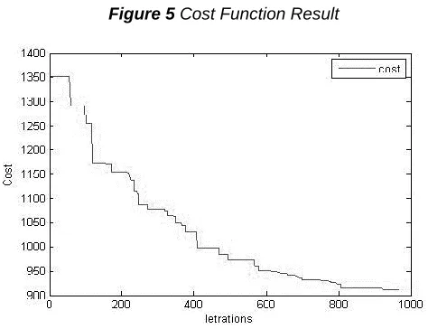
Also this graph show the decreasing the cost function with the iterations used.

Figure 5 Cost Function Result

7

C

In this paper a combinatorial model associated with a metaheuristic technique for solving the TNERPP problem using DC-TNEP prior to AC-TNEP model for a transmission expansion system is presented. Despite the fact that the proposed metaheuristic can find better solution than CGA but the main contribution of this paper is to propose an efficient approach with less effort for transmission network planning when using AC model. Although it is possible to solve the TNERPP in one stage, the easiest and by far the fastest way is to start with the solution of a DC model and then reinforce the expanded transmission network using new transmission lines as well as reactive power sources. A new methodology is also proposed to solve the reinforcement stage in two steps: the transmission network is reinforced with new lines and then with reactive power sources. The ordinary genetic algorithm and the Chaotic DEA are used to solve different steps of the TNERPP problem. A set of examples using a modified Garver system and a general analysis of the results are presented. In this case we will find that the results of the two algorithms are close in matter of fact the different is small although the CDE shows its ability in decreasing the power loss of the whole system. Also a slightly decreasing in the cost , on the other hand the load on the line decreases, according to the application we use we can change the methodology of

optimization and this will be presented in more further future work.

R

[1] T. Sum-Im, G. A. Taylor, M. R. Irving, and Y. H. Song, ―Differential evolution algorithm for static and multistage transmission expansion planning,‖ IET Gener. Transm. Distrib., vol. 3, no. 4, p. 365, 2009.

[2] M. Rahmani, M. Rashidinejad, E. M. Carreno, and

R. Romero, ―Efficient method for AC transmission network expansion planning,‖ Electr. Power Syst. Res., vol. 80, no. 9, pp. 1056–1064, 2010.

[3] C. Deng, C. Liang, B. Zhao, Y. Yang, and A. Deng, ―Structure-Encoding Differential Evolution for Integer Programming,‖ J. Softw., vol. 6, no. 1, pp. 140–147, 2011.

[4] L. D. S. Coelho, ―Reliability-redundancy

optimization by means of a chaotic differential evolution approach,‖ Chaos, Solitons and Fractals, vol. 41, no. 2, pp. 594–602, 2009.

[5] W. Liang, L. Zhang, and M. Wang, ―The chaos differential evolution optimization algorithm and its application to support vector regression machine,‖ J. Softw., vol. 6, no. 7, pp. 1297–1304, 2011.

[6] A. Mahmoudabadi, M. Rashidinejad, and M.

Zeinaddini-Maymand, ―A New Model for

Transmission Network Expansion and Reactive Power Planning in a Deregulated Environment,‖ Engineering, vol. 04, no. 02, pp. 119–125, 2012.

[7] a. Verma, B. K. Panigrahi, and P. R. Bijwe, ―Transmission network expansion planning with adaptive particle swarm optimization,‖ 2009 World Congr. Nat. Biol. Inspired Comput., pp. 1099–1104, 2009.

[8] G. D. Dhole and M. D. Khardenvis, ―Dynamic Transmission Network Expansion Planning,‖ vol. 3, no. 6, pp. 114–117, 2015.

[9] R. Mínguez and R. García-Bertrand, ―Robust