Recent Developments in Few-Nucleon Scattering

Recent Developments in Few-Nucleon Scattering

Istituto Nazionale di Fisica Nucleare, Largo B. Pontecorvo 3, 56127 (Pisa), Italy

Abstract. Using modern nucleon-nucleon interactions in the description of the A=3,4 nuclei, it is not possible to reproduce both the three- and four-nucleon binding energies simultaneously. This is one manifestation of the necessity of including a three-nucleon force in the nuclear Hamiltonian. Several models of the three-nucleon force exist and are applied in the description of light nuclei. However, as it is discussed here, a simultaneous description of the three- and four-body binding energies and the n−d doublet scattering length seems to be problematic. Accordingly, a comparative study of some of these models is performed. In a different analysis, we study applications of the Kohn Variational Principle, formulated in terms of integral relations, to describe N₋d scattering processes.

1 Introduction

Realistic nucleon-nucleon (NN) potentials reproduce the experimental NN scattering data up to energies of 350 MeV with aχ2 _{per datum close to 1. However, the use of these} potentials in the description of the three- and four-nucleon bound and scattering states gives a χ2 per datum much larger than 1 (see for example Refs.[1, 2]). In order to im-prove that situation, different three-nucleon force (TNF) models have been introduced so far. Widely used in the literature are the Tucson-Melbourne (TM) and the Urbana IX (URIX) models [3, 4]. These models are based on the exchange mechanism of two pions between three nucle-ons with the intermediate excitation of a∆resonance. The TM model has been revisited within a chiral symmetry ap-proach [5], and it has been demonstrated that the contact term present in it should be dropped. This new TM poten-tial, known as TM′_{, has been subsequently readjusted [6].} The final operator structure coincides with that one given in the TNF of Brazil already derived many years ago [7]. Recently, TNFs have been derived based on chiral effective field theory at next-to-next-to-leading order [8]. A local version of these interactions (hereafter referred as N2LOL) can be found in Ref. [9]. All these models contain a certain number of parameters that fix the strength of the interac-tion. It is a common practice to determine these parameters from the three- and four-nucleon binding energies. A par-ticular TNF is in general associated to a specific NN poten-tial and the sum of the two interactions forms the nuclear potential energy. The two- and three-nucleon interactions derived using chiral effective field theory are consistently constructed. However a particular TNF can be used asso-ciated with different NN interactions. As a consequence, the parametrization of a particular TNF could change since different NN potentials predict different A = 3,4 binding energies.

a _{e-mail:[email protected]}

More recently, a new class of two-nucleon interactions has been obtained (Vlow−kpotentials). With the purpose of

eliminating the high-momentum part of the interaction, the Hilbert space has been separated into low and high mo-mentum regions and the renormalization group method has been used to integrate out the high momentum components above a cutoffΛ[10]. The value forΛis typically chosen to reproduce the triton binding energy.

All these potential models can be used to study bound and scattering states in the A = 3,4 systems in order to extract information about their capability to describe the nuclear dynamics. Besides the bound state energies, in the

A = 3 system, the n₋d doublet scattering length 2_a

nd

can give valuable information. In principle this quantity is correlated, to some extent, to the A = 3 binding energy through the so-called Phillips line [11, 12]. However the presence of TNFs of the type studied here breaks this cor-relation. Therefore2_a

ndemerges as an independent

observ-able. Due to the lack of excited states in the A=3 system, the zero energy state is the first one above the ground state. In the case of n₋d scattering at zero energy, the J = 1

2

+

state is orthogonal to the triton ground state and, for this reason, it presents a node in the relative distance between the incident nucleon and the deuteron. The position of the node is related to the scattering length and it is also sen-sitive to the relation between the overall attraction and re-pulsion of the interaction. Several of the realistic NN po-tentials underestimate the triton binding energy. Therefore by adding a TNF, with the strength fixed for example to re-produce the triton binding energy, the balance between the total attraction and repulsion in the potential changes. This leads to a modification in 2_a

nd and this modification

de-pends on the parameters in the TNF. The determination of the TNF parametrization able to describe the triton binding energy B(3_{H), theα-particle binding energy B(}4_{He) and} 2_a

ndhas been analyzed in Ref. [8] for a TNF derived from

DOI:10.1051/epjconf/20100301002

chiral effective field theory. A similar analysis has not been done for the local TNF models URIX, TM’ and N2LOL.

In Refs. [13, 14] results for B(3_{H), B(}4_He), 2_a

nd are

given using different combinations of NN interactions (see Table 1). Those results indicate that the models are not able to describe simultaneously the A = 3,4 binding en-ergies and2and. In order to analyze further the mentioned

discrepancies, here we study potential models constructed summing to the AV18 NN potential [15] the three-nucleon interactions of TM’, URIX and N2LOL. Parametrizations of the URIX and TM’ models already exist in conjunc-tion with the AV18 potential. Conversely the N2LOL force has been constructed using the N3LO-Idaho potential from Entem et al. [16]. So, here we adapt its parametrization to reproduce, when summed to the AV18 interaction, the tri-ton binding energy. Different parametrizations of the three TNF models are analyzed studying the description of B(3H),

B(4_{He) and}2_a

ndand some polarization observables in p−d

scattering. The calculations have been done using the hy-perspherical harmonic (HH) method as given in Refs. [17– 20] to describe bound and scattering states in A=3,4 sys-tems using local potentials. The extension to treat nonlocal potentials was given in Refs. [14, 21].

In a different application devoted to study scattering states in few-nucleon systems, a discussion of the use of the integral relations derived in Ref. [22] from the Kohn Variational principle (KVP) is given. It has been shown that starting from the KVP, the tangent of the phase-shift can be put in a form of a quotient where both, the nu-merator and the denominator, are given in the form of an integral relation. This is similar to what was proposed in Ref. [23], however its strict relation with the KVP has not been recognized. To be noticed that a general formulation of the scattering theory using surface-integrals is given in Ref. [24]. Here we would like to discuss some specific examples of the integral relations derived from the KVP. Starting the analysis in the simplest case, the A = 2 sys-tem, we show that they can be used to compute phase-shifts from bound state like functions. A second application of the integral relations regards the possibility of determin-ing phase-shifts from a calculation in which the Coulomb potential has been screened. All these examples serve to demonstrate the general validity of the KVP formulated in terms of integral relations. Due to their short-range nature, they are determined by the wave function in the interaction region and not from its explicit asymptotic behaviour. This means that each wave function solving (H₋E)Ψ=0 in the interaction region can be used to determine the correspond-ing scattercorrespond-ing amplitude even if its asymptotic behaviour is not the physical one.

2 The HH expansion for

A

₌

3

,

4

systems

In this section we briefly review the HH method for bound and scattering states.

2.1 The HH Method for Bound States

The nuclear wave function for the three-body system can be written as

|Ψ_i=X

µ

cµ|Ψµi, (1)

where_|Ψµiis a suitable complete set of states, andµis an index denoting the set of quantum numbers necessary to completely specify the basis elements.

The coefficients of the expansion can be calculated us-ing the Rayleigh-Ritz variational principle, which states that

hδcΨ|H−E|Ψi=0, (2)

where δcΨ indicates the variation of Ψ for arbitrary

in-finitesimal changes of the linear coefficients cµ. Where the Hamiltonian of the system consists in the kinetic part plus two- and three-nucleon interaction terms

H=−~ 2 2m

X

i

∇2

i +

X

i<j

V(i,j)+ X

i<j<k

W(i,j,k) (3)

The problem of determining cµand the energy E is re-duced to a generalized eigenvalue problem,

X

µ′

hΨµ|H−E|Ψµ′ic_µ′=0. (4)

The main difficulty of the method is to compute the ma-trix elements of the Hamiltonian H with respect to the ba-sis states_|Ψµi. Usually H is given as a sum of terms (ki-netic energy, two-body potential, etc.). The calculation of the matrix elements of some parts of H can be more con-veniently performed in coordinate space, while for other parts it could be easier to work in momentum space. There-fore, it is important that the basis states_|Ψµihave simple expressions in both spaces. The HH functions indeed have such a property.

In the case of three nucleons of mass m the Jacobi vec-tors x1p,x2p correspond to a given particle permutation denoted with p, which specifies the particle order i,j,k,

x2p= 1 √ 2

(rj−ri),

x1p=

r

2 3(rk−

1

2(ri+rj)). (5) Here p=1 corresponds to the order 1,2,3. It is convenient to replace the modulii of x2p andx1p with the so-called hyperradius and hyperangle, defined as

ρ= qx2 1p+x

2

2p, (6)

tanφp=

x1p

x2p

. (7)

Note that ρdoes not depend on the particle permutation

p. The complete set of hyperspherical coordinates is then

given by_{ρ, Ω(ρ)p }, with

and the suffix (ρ) recalls the use of the coordinate space. The expansion states_|Ψµiof Eq. (1) are then given by

|Ψµ(ρ)i= fl(ρ)Y_{G_}(Ω(ρ)), (9)

where fl(ρ) for l=1, . . .M is a complete set of hyperradial

functions, chosen of the form

fl(ρ)=γ3 s

l!

(l+5)! L (5)

l (γρ) e−

γ

2ρ. (10)

Here L(5)_l (γρ) are Laguerre polynomials, and the non-linear parameterγis variationally optimized. As an example, for the N3LO-Idaho potential, it can be chosen in the interval 6–8 fm−1_.

The functions_Y{G_}(Ω(ρ)) are written as

Y{G_}(Ω(ρ))=

3

X

p=1

"

YLLz [G](Ω

(ρ)

p )⊗[S2⊗

1 2]S Sz

#

J Jz [T2⊗

1 2]T Tz,

(11) where the sum is performed over the three even permuta-tions. The spin (isospin) of particles i and j are coupled to S2(T2), which is itself coupled to the spin (isospin) of the third particle to give the state with total spin S (isospin

T,Tz). The total orbital angular momentum L and the

to-tal spin S are coupled to the toto-tal angular momentum J,Jz.

The functions YLLz [G](Ω

(ρ)

p ), having a definite value of L,Lz,

are the HH functions:

YLLz [G](Ω

(ρ)

p )=

"

Yℓ2( ˆx2p)⊗Yℓ1( ˆx1p)

#

LLz

N[G](2)Pℓn1,ℓ2(φp).

(12) Here Yℓ1( ˆx1p) and Yℓ2( ˆx2p) are spherical harmonics, N[G] is a normalization factor and(2)Pℓ1,ℓ2

n (φp) is an

hyperspher-ical polynomial. The grand angular quantum number G is defined as G=2n+ℓ1+ℓ2. The notations [G] and{G}of Eqs. (12) and (11) stand for [ℓ1, ℓ2; n] and{ℓ1, ℓ2,L,S2,T2,

S,T ; n_}, respectively, andµof Eq. (9) isµ = {G_},l. Note

that each set of quantum numbers_{ℓ1, ℓ2,L,S2,T2,S,T}is called “channel”, and the antisymmetrization of_Y{G}(Ω(ρ)) requiresℓ2+S2+T2to be odd. In addition,ℓ1+ℓ2must be even (odd) for positive (negative) parity.

The HH functions having grand angular quantum num-ber G constructed in terms of a given set of Jacobi vec-torsx1p,x2p, defined starting from the particle order i,j,k, can always be expressed in terms of the HH functions con-structed, for instance, in terms ofx1(p=1),x2(p=1)with the same value of G. In fact, the following relation holds

YLLz [ℓ1,ℓ2;n](Ω

(ρ)

p )=

X

ℓ′ 1,ℓ′2,n′

a(p),_ℓ L

1,ℓ2,n;ℓ1′,ℓ′2,n′Y

LLz [ℓ′

1,ℓ′2;n′](Ω (ρ)

(p=1)), (13)

where the sum is restricted to the valuesℓ′₁,ℓ₂′, and n′such thatℓ′₁+ℓ′₂+2n′=G. The coefficients a(p),_ℓ L

1,ℓ2,n;ℓ′1,ℓ2′,n′ relat-ing the two sets of HH functions are known as the Raynal-Revai coefficients [25]. Also the spin-isospin states can be recoupled to obtain states where the spin and isospin quan-tum numbers are coupled in a given order of the particles.

The result is that the antisymmetric functions_Y{G} can be expressed as a superposition of functions constructed in terms of a given order of particles i,j,k, each one having

the pair i, j in a definite spin and angular momentum state. When the two-body potential acts on the pair of particles

i, j, the effect of the projection is easily taken into account. The expansion states of Eq. (1) in momentum space can be obtained as follows. Let~_k1p,~_{k2pbe the conjugate}

Jacobi momenta of the Jacobi vectors, given by

~_{k2p= √}1

2(pj−pi),

~_k1p= r

2 3(pk−

1

2(pi+pj)), (14)

pibeing the momentum of the i-th particle. We then define

a hypermomentum Q and a set of angular-hyperangular variables as

Q= qk2 1p+k

2 2p,

Ω(Q)_p =[ ˆk2p,kˆ1p;ϕp], (15)

where

tanϕp=

k1p

k2p

. (16)

Then, the momentum-space version of the wave function given in Eq. (9) is

|Ψ_µ(Q)_i=gG,l(Q)Y_{G_}(Ω(Q)), (17)

where_Y{G_}(Ω(Q)) is the same asY_{G_}(Ω(ρ)) of Eq. (11) with xip→kip, and

gG,l(Q)=(−i)G

Z _∞

0

dρ ρ

3

Q2 JG+2(Qρ) fl(ρ). (18) With the adopted form of fl(ρ) given in Eq. (10), the

cor-responding functionsgG,l(Q) can be easily calculated, and

they are explicitly given in Ref. [21].

2.2 The HH Method for Scattering States Below Deuteron Breakup Threshold

We consider here the extension of the HH technique to describe N₋d scattering states below deuteron breakup

threshold, when both local and non-local interaction mod-els are considered.

The wave functionΨLS J Jz

N₋d describing the N−d

scatter-ing state with incomscatter-ing orbital angular momentum L and channel spin S , parityπ=(₋)L, and total angular momen-tum J,Jz, can be written as

ΨLS J Jz

N−d =Ψ

LS J Jz

C +Ψ

LS J Jz

A , (19)

whereΨLS J Jz

C describes the system in the region where the

particles are close to each other and their mutual interac-tions are strong, whileΨLS J Jz

A describes the relative motion

region, where the N₋d nuclear interaction is negligible.

The functionΨLS J Jz

C , which has to vanish in the limit of

large intercluster separations, can be expanded on the HH basis as it has been done in the case of bound states. There-fore, applying Eq. (1), the functionΨLS J Jz

C can be casted in

the form

|ΨLS J Jz

C i=

X

µ

cµ|Ψµi, (20)

where_|Ψµiis defined in Eqs. (9) and (17) in coordinate-and momentum-space, respectively.

The functionΨLS J Jz

A is the appropriate asymptotic

solu-tion of the relative N₋d Schr¨odinger equation. It is written

as a linear combination of the following functions,

Ωλ_{LS J J}

z= 3

X

p=1

Ωλ_{LS J J}

z(p), (21)

where the sum over p has to be done over the three even permutations and

Ωλ_{LS J J}

z(p)=

X

l=0,2

wl(x2p) RλL(yp)

[Yl( ˆx2p)⊗S2]1⊗ 1 2

S

⊗YL( ˆyp)

J Jz [T2⊗

1

2]T Tz. (22)

Here the spin and isospin quantum numbers of particles

i and j have been coupled to S2 and T2, with S2 = 1,

T2=0 for the deuteron,wl(x2p) is the deuteron wave func-tion component in the waves l = 0,2,yp is the distance

between N and the center of mass of the deuteron, i.e.

yp = q

3

2x1p, Yl( ˆx2p) and YL( ˆyp) are the standard spher-ical harmonic functions, and the functions Rλ

L(yp) are the

regular (λ_≡R) and irregular (λ_≡I) radial solutions of the

relative two-body N₋d Schr¨odinger equation without the

nuclear interaction. These regular and irregular functions, denoted as_FL(yp) andGL(yp) respectively, have the form

FL(yp)=

1 (2L+1)!!qL_C

L(η)

FL(η, ξp)

ξp

,

GL(yp)=(2L+1)!!qL+1CL(η) fR(yp)

GL(η, ξp)

ξp

, (23)

where q is the modulus of the N₋d relative momentum

(related to the total kinetic energy in the center of mass system by Tcm =

q2

2µ, µbeing the N−d reduced mass),

η =2µe2/q andξp =qyp are the usual Coulomb

parame-ters, and the regular (irregular) Coulomb function FL(η, ξp)

(GL(η, ξp)) and the factor CL(η) are defined in the standard

way [26]. The factor (2L+1)!!qL_C

L(η) has been introduced

so that_F and_Ghave a finite limit for q_→0. The function

fR(yp) =[1−exp(−byp)]2L+1has been introduced to

reg-ularize GLat small values ofyp. The trial parameter b is

determined by requiring that fR(yp)→1 outside the range

of the nuclear interaction, thus not modifying the asymp-totic behaviour of the scattering wave function. A value of b = 0.25 fm−1 _{has been found appropriate. The} non-Coulomb case of Eq. (23) is obtained in the limit e2

→0.

In this case, FL(η, ξp)/ξp and GL(η, ξp)/ξp reduce to the

regular and irregular Riccati-Bessel functions and the fac-tor (2L+1)!!CL(η)→1 forη→0.

With the above definitions,ΨLS J Jz

A can be written in the

form

ΨLS J Jz

A =

X

L′S′

"

δLL′δS S′ΩR_L′S′J Jz+R

J

LS,L′S′(q)ΩIL′S′J Jz

#

,

(24) where the parameters_RJ

LS,L′S′(q) give the relative weight between the regular and irregular components of the wave function. They are closely related to the reactance matrix (_K-matrix) elements, which can be written as

KJ

LS,L′S′(q)=

(2L+1)!!(2L′_{+1)!! q}L+L′₊₁

CL(η)CL′(η)RJ_LS,L′_S′(q)(25).

By definition of the_K-matrix, its eigenvalues are tanδLS J,

δLS J being the phase shifts. The sum over L′ and S′ in

Eq. (24) is over all values compatible with a given J and parityπ. In particular, the sum over L′_{is limited to include} either even or odd values since (₋1)L′

=π.

The matrix elements_RJ_LS,L′S′(q) and the linear coeffi -cients cµoccurring in the expansion ofΨ_CLS J Jz of Eq. (20) are determined applying the Kohn variational principle, which states that the functional

[_RLSJ _,L′_S′(q)]=RJ_LS,L′_S′(q)−

D

ΨL′S′J Jz

N₋d |L|Ψ

LS J Jz

N₋d E

,

L= m

2√3~2(H−E), (26)

has to be stationary with respect to variations of the trial parameters inΨLS J Jz

N−d . Here E is the total energy of the

sys-tem, m is the nucleon mass, and_Lis chosen so that hΩR_{LS J J}

z|L|Ω

I

LS J Jzi − hΩ

I

LS J Jz|L|Ω

R

LS J Jzi=1. (27)

As described in Ref. [18], using Eqs. (20) and (24), the variation of the diagonal functionals of Eq. (26) with re-spect to the linear parameters cµleads to the following sys-tem of linear inhomogeneous equations:

X

µ′

hΨµ|L|Ψµ′icµ′=−Dλ_{LS J J}

z(µ). (28)

Two different terms Dλcorresponding toλ _≡ R,I are

in-troduced and are defined as

Dλ_{LS J J}

z(µ)=hΨµ|L|Ω λ

LS J Jzi. (29)

The matrix elements _RJ_LS,L′S′(q) are obtained varying the diagonal functionals of Eq. (26) with respect to them. This leads to the following set of algebraic equations

X

L′′S′′

RJLS,L′′_S′′(q)XL′_S′_,L′′_S′′ =Y_LS,L′_S′, (30)

with the coefficients X and Y defined as

XLS,L′S′ =hΩI_{LS J J} z+Ψ

LS J Jz,I

C |L|Ω

I L′S′J Jzi,

YLS,L′_S′ =−hΩR_{LS J J} z+Ψ

LS J Jz,R

C |L|Ω

I

Here ΨLS J Jz,λ

C is the solution of the set of Eq. (28) with

the corresponding Dλ _{term. A second order estimate of} RJ

LS,L′S′(q) is given by the quantities [RLSJ ,L′S′(q)], obtained by substituting in Eq. (26) the first order results. Such second-order calculation provides a symmetric reactance matrix. This condition is not a priori imposed, and therefore it is a useful test of the numerical accuracy.

In the particular case of q=0 (zero-energy scattering), the scattering can occur only in the channel L=0 and the observables of interest are the scattering lengths. Within the present approach, they can be easily obtained from the relation

(2J+1)_a

Nd=−lim

q→0R

J

0J,0J(q). (32) An alternative way to solve the scattering problem, used when q,0, is to apply the complex Kohn variational prin-ciple to the_S-matrix, as in Ref. [18].

The approach presented so far for bound and scattering states does not have too many differences compared to the method presented for instance in Ref. [17], and known as pair-correlated hyperspherical harmonics (PHH) method. In fact, in the PHH method a correlation factor is included in the HH expansion of Eq. (20) to take into account the strong short-range correlations induced by the realistic two-body potentials, like the AV18. The presence of correlation functions makes the convergence of the expansion much faster than in the uncorrelated case. However, the PHH method cannot be simply implemented when non-local two-body interactions are considered, unless the Fourier trans-form of the potential is pertrans-formed. The calculation involv-ingΨLS J Jz

C can be performed with the HH or PHH

expan-sions in coordinate- or in momentum-space, depending on what is more convenient.

3 Three Nucleon Force Models

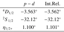
In Ref. [13] the description of bound states and zero-energy states for A=3,4 has been reviewed in the context of the HH method. In Table 1 we report results for the triton and 4_{He binding energies as well as for the doublet n}

−d

scatter-ing length2_a

nd using the AV18 and the N3LO-Idaho NN

potentials and using the following combinations of two-and three-nucleon interactions: AV18+URIX, AV18+TM’, N3LO-Idaho+N2LOL and N3LO-Idaho+URIXp. In this last model the parameter in front of the spisospin in-dependent part of the URIX potential has been rescaled by a factor of 0.384 to fit the triton binding energy [14] (we call this model URIXp). We have considered also the Vlowk

model, obtained from the AV18 interaction with a cutoff

parameterΛ =2.2 fm−1_{. The results are compared to the} experimental values reported in the table. Worthy of notice is the recent very accurate datum for2and[27].

From the table we may observe that only the results ob-tained using an interaction model that includes a TNF are close to the corresponding experimental values. In the case of the AV18+TM’, the strength of the TM’ potential has been fixed to reproduce the4He binding energy and, as can be seen from the table, the triton binding energy is under-predicted. Conversely, the strength of the URIX potential

Table 1.The triton and4_{He binding energies B (in MeV), and}

doublet scattering length2_a

nd(in fm) calculated using the indi-cated two- and three-nucleon interactions. The experimental re-sults are also reported.

Potential B(3_{H) B(}4_He) 2_and

AV18 7.624 24.22 1.258

N3LO-Idaho 7.854 25.38 1.100

AV18+TM’ 8.440 28.31 0.623

AV18+URIX 8.479 28.48 0.578

N3LO-Idaho+N2LOL 8.474 28.37 0.675

N3LO-Idaho+URIXp 8.481 28.53 0.623

Vlow−k 8.477 29.15 0.572

Exp. 8.482 28.30 0.645±0.003±0.007

has been fixed to reproduce the triton binding energy giv-ing too much bindgiv-ing for4_{He. The strength of the N2LOL} potential has been fixed to reproduce simultaneously the triton and the 4He binding energies whereas the N3LO-Idaho+URIXp model overbinds 4_{He. These two models} give a better description of2_a

nd. The Vlow₋kinteraction

re-produces the triton binding energy but overbinds4He ap-preciably and2and is not well described. In conclusion a

simultaneous correct description of the three quantities is not achieved by any of the models considered.

To analyze further this fact, we give a brief description of the TM’ (or Brazil), URIX and N2LOL models. They can be put in the following way:

W(1,2,3)=aWa(1,2,3)+bWb(1,2,3)+dWd(1,2,3)

W(1,2,3)=aWa(1,2,3)+bWb(1,2,3)+dWd(1,2,3)

+cDWD(1,2,3)+cEWE(1,2,3). (33)

Each term corresponds to a different source and has a dif-ferent operator structure. The first three terms arise from the exchange of two pions between three nucleons. The

a-term is coming fromπN S -wave scattering whereas the b-term and d-term, which are the most important, come

from πN P-wave scattering. The specific form of these

three terms in configuration space is the following:

Wa(1,2,3)=

W0

c2_~2(τ1·τ2)(σ1·r31)(σ2·r23)y(r31)y(r23)

Wb(1,2,3)=W0(τ1·τ2)[(σ1·σ2)y(r31)y(r23)

+(σ1·r31)(σ2·r23)(r31·r23)t(r31)t(r23)

+(σ1·r31)(σ2·r31)t(r31)y(r23)

+(σ1·r32)(σ2·r32)y(r31)t(r23)] (34)

Wd(1,2,3)=W0(τ3·τ1×τ2)[(σ3·σ2×σ1)y(r31)y(r23)

+(σ1·r31)(σ2·r23)(σ3·r31×r23)t(r31)t(r23)

+(σ1·r31)(σ2·r31×σ3)t(r31)y(r23)

following function

f0(r)= 12π

m3π 1 2π2

Z _∞

0

dqq2 j0(qr) q2_+m2

π

FΛ(q) (35)

where mπis the pion mass and

  

y(r)= 1

rf0′(r)

t(r) = 1ry′(r) .

(36)

The cutofffunction FΛin the TM’ or Brazil models is taken as [(Λ2_−m2

π)/(Λ2+q2)]2. In the N2LOL model it is taken as exp(₋q4/Λ4). The momentum cutoffΛis a parameter of the model fixing the scale of the problem in momentum space. In the N2LOL, it has been takenΛ= 500 MeV, whereas in the TM’ model the quantityΛ/mπ has been varied to describe the triton or4_{He binding energy at fixed values of} the constants a,b and d. In the literature several cases have been explored with typical values aroundΛ=5mπ.

In the URIX model the radial dependence of the b- and

d-terms is given in terms of the functions

  

Y(r)=e−x_/xξ Y

T (r)=(1+3/x+3/x2_)Y(r)ξ

T

(37)

with x=mπr and the cutofffunctions are defined asξY =

ξT =(1−e−cr

2

), with c=2.1 fm−2. This regularization has been used in the AV18 potential as well. Since the param-eters in the URIX model has been determined in conjunc-tion with the AV18 potential, the use of the same regular-ization was a choice of consistency. The relation between the functions Y(r),T (r) and those of the previous models

is _

 

Y(r) =y(r)+T (r)

T (r)= r32t(r) .

(38)

With the definition given in Eq.(35), the asymptotic be-haviour of the functions f0(r),y(r) and t(r) is:

f0(r→ ∞)→ 3

m2 π

e−x

x

y(r_{→ ∞}) _{→ −}3e −x

x2 1+ 1

x

!

(39)

t(r_{→ ∞}) _→ 3

r2 e−x

x 1+

3 x+ 3 x2 ! .

In fact, with the normalization chosen for f0, the functions

Y and T defined fromyand t in Eq. (38) and those ones de-fined in the URIX model in Eq. (37) coincide at large sep-aration distances. Conversely, they have a different short range behavior.

The last two terms in Eq. (33) correspond to a 2N con-tact term with a pion emitted or absorbed (D-term) and to a 3N contact interaction (E-term). Their local form, in con-figuration space, derived from Ref. [9], are

WD(1,2,3)=W0D(τ1·τ2)×

{(σ1·σ2)[y(r31)Z0(r23)+Z0(r31)y(r23)]

+(σ1·r31)(σ2·r31)t(r31)Z0(r23)

+(σ1·r32)(σ2·r32)Z0(r31)t(r23)} (40)

WE(1,2,3)=W0E(τ1·τ2)Z0(r31)Z0(r23). The constant WD

0,W

E

0 fix the strength of these terms. In the case of the URIX model the E-term is present without the isospin operator structure and it has been included as purely phenomenological, without justifying its form from a particular exchange mechanism. Its radial dependence has been taken as Z0(r) = T2(r). In the N2LOL model, the function Z0(r) is defined as

Z0(r)= 12π

m3π 1 2π2

Z ∞

0

dqq2j0(qr)FΛ(q) (41)

with the same cutofffunction used in the definition of f0in Eq.( 35), FΛ(q)=exp(−q4/Λ4). In the TM’ model the D-and E-terms are absent.

Each model is now identified from the values assigned to the different constants a,b,d,cD,cE. Following Refs. [6,

28], in the case of the TM’ model, the values of the con-stants have been chosen as a=−0.87 m−1

π , b=−2.58 m−π3, and d =−0.753 m−3

π ; the strength W0 =(gmπ/8πmN)2 m4π and the cutoffhas been fixed toΛ=4.756 mπin order to describe correctly B(4_{He). In Table 1 the calculations have} been done using these values withg2_{=197.7, m}

π=139.6 MeV, mN/mπ=6.726 (mNis the nucleon mass) as given in

the original derivation of the TM potential. As mentioned before, this model does not include the D- and E-terms.

In the URIX model the b- and d-terms are present, however with a fix relative value. The strength of these terms is: bW0=4 APW_2π and d=b/4, with APW_2π =−0.0293 MeV. The model includes a purely central repulsive term introduced to compensate the attraction of the previous term, which by itself would produce a large overbinding in infinite nuclear matter. It is defined as

W_EURIX(1,2,3)=ART2(r31)T2(r23) (42) with AR=0.0048 MeV.

In the N2LOL potential the constants of the a-, b-, d-,

D- and E-terms are defined in the following way:

W0= _12π12

mπ Fπ 4 g2 Am 2 π

W_D0 =12π12

_m π

Fπ 4_m

π

Λx

_gAmπ

8 (43) W0 E = 1 12π2 _mπ Fπ

4_m

π

Λx

mπ

with a = c1m2π, b = c3/2, d =c4/4, and c1 = −0.00081 MeV−1_{, c}

3 =−0.0032 MeV−1, c4=−0.0054 MeV−1taken from Ref. [16]. The other two constants, cD = 1.0 and

cE =−0.029, have been determined in Ref. [9] from a fit to

B(3H) and B(4He) using the N3LO-Idaho+N2LOL poten-tial model. The numerical values of the constant entering in W0, W0_Dand W_E0are taken as mπ =138 MeV, Fπ =92.4 MeV,gA =1.29, and the chiral symmetry breaking scale

Λx=700 MeV.

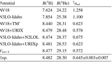
functions Z0(r),y(r) and T (r) for the three models under consideration. In the TM’ model using the definition of Eq.(41) and using the corresponding cutofffunction we can define:

Z₀T M(r)= 12π

m3 π

1 2π2

Z ∞

0

dqq2j0(qr)

Λ2₋m2 π

Λ2_+q2

!2

= 3

2

_mπ

Λ

_Λ2

m2 π

−1

!2

e−Λr . (44)

This function is showed in the first panel of Fig. 1 as a dashed line. From the figure we can see that, in the case of the URIX model, the functions Z0(r) andy(r) go to zero as

r_→0. This is not the case for the other two models and is a consequence of the regularization choice of the Y and T functions adopted in the URIX.

4 Parametrization Study of the Three

Nucleon Forces

In this section we study possible variations to the parametriza-tion of the TNF models in order to describe the A =3,4 binding energies and2and.

4.1 Tucson-Melbourne Force

We first study the TM’ potential and we would like to see if, using the AV18+TM’ interaction, it is possible to repro-duce simultaneously the triton binding energy and the dou-blet n₋d scattering length for some values of the

param-eters. The a-term gives a very small contribution to these quantities, therefore, in the following analysis we maintain it fixed at the value a=−0.87 m−1

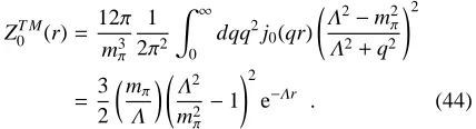
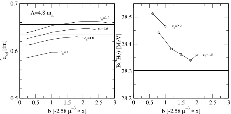
π . In Fig. 2, left panel, the doublet n₋d scattering length is given as a function of the

parameter b (in units of its original value b =−2.58 m−π3) for different values of the cutoffΛ(in units of mπ). The box in the figure includes values compatible with the ex-perimental results. The value of the constant d has been fixed to reproduce the triton binding energy. The corre-sponding values of the parameter d (in units of its original value d = −0.753 m−3

π ) are given in the right panel as a function of b. Each point of the curves in both panels cor-responds to a set of parameters that, in connection with the AV18 potential, reproduces the triton binding energy. The variations of the parameters given in Fig. 2 do not exhaust all the possibilities. However we can observe that, with the AV18+TM’ potential, there is a very small region in the parameter’s phase space available for a simultaneous de-scription of the triton binding energy and the doublet scat-tering length. This small region corresponds to a big value of b and d results to be almost zero. Moreover, the value of the cutoffΛaround 3.8mπis smaller than the values usually used with the TM’ potential (Λ_≈5mπ).

To be noticed that, for negative values of the parame-ters a, b and d, the TM’ potential is attractive. It does not include explicitly a repulsive term. Added to a specific NN

potential that underpredicts the three-nucleon binding en-ergy, it supplies the extra binding by fixing appropriately its strength. However, as mentioned in the Introduction, the scattering length is sensitive to the balance between the at-tractive part and the repulsive part of the complete interac-tion. Therefore, it seems that supplying only an attraction, fixed to reproduce the triton binding energy, in the case of the TM’ interaction it is difficult to reproduce correctly this balance.

As discussed before, the TM’ potential is a modifica-tion of the original TM potential compatible with chiral symmetry. At the same order (next-to-next-to-leading or-der) in the chiral effective field theory the D- and E-terms appear (see Ref. [8] and references therein) as given in Eq.(33). Here we introduce the following additional term to the TM’ potential based on a contact term of three nu-cleons

WT M_E (1,2,3)=W_E0X

cyc

Z₀T M(r31)Z0T M(r23). (45)

This term is similar to the repulsive term of the URIX model and, for the sake of simplicity, we do not include the (τ1·τ2) operator. The function Z₀T Mis a positive function, therefore, for positive values of cE, the new term is

repul-sive. We include it in the following analysis of the TM’ potential. The analysis of the new term is given in Fig. 3. In the left panel the doublet n₋d scattering length is given

as a function of the parameter b (in units of its original value b =−2.58 m−_π3) for different values of the strength of the W_ET M-term. The value of the cutoffΛhas been fixed to 4.8 mπ. The box in the figure includes values compat-ible with the experimental results. Moreover, the value of the constant d has been fixed to reproduce the triton bind-ing energy. The correspondbind-ing values of the 4He binding energy, B(4He), is given in the right panel.

Comparing the left panels in Figs. 2 and 3, the effect of the new term is clear. In Fig. 2 we see that usingΛ =

4.8 mπ,2and is not well reproduced. Conversely, in Fig. 3,

the inclusion of the new term moves this curve in the cor-rect dicor-rection and with values of its strength around cE =

1.6 it is possible to reproduce the experimental value of 2_a

nd. There is also an improvement in the description of

B(4_{He). In fact, the AV18+TM’ model withΛ = 4.8 m} π reproduces the triton binding energy as can be seen from Fig. 2. However it predicts B(4He)=28.55 MeV, which is slightly too high. With the W_ET M-term, at cE = 1.6, the

description of B(4_{He) improves. For example with b =} −3.87 m−3

π , d = −3.375 mπ−3 and Λ = 4.8 mπ, we ob-tain B(4He) =28.36 MeV, very close to the experimental value.

4.2 UrbanaIX Force

In the following we analyze the URIX potential which has two parameters, APW

2π and AR. In this model the strength of the d-term was related to the strength of the b-term as

0 1 2 3 4 5 r [fm]

0 50 100 150

Z 0

(r)

0 1 2 3 4 5

r [fm] -45

-30 -15 0

y(r)

0 1 2 3 4 5

r [fm] 0

5 10 15

T(r)

Fig. 1.The Z0(r),y(r) and T (r) functions as functions of the interparticle distance r for the URIX (solid line), TM’ (dashed line) and

N2LOL (dotted line) models.

0 0.5 1 1.5 2 2.5 3 3.5 4

b [-2.58µ−3] 0.55

0.6 0.65

2 a

nd

[fm]

0 0.5 1 1.5 2 2.5 3 3.5 4

b [-2.58µ−3] 0

2 4 6 8

d[-0.753

µ

−3 ]

Λ=5.4Λ=5.2

Λ=5.0Λ=4.8

Λ=4.6 Λ=4.4

Λ =4.2 Λ=4.0

Λ=3.8

Λ=4.8 Λ=3.8

Fig. 2.The doublet scattering length an₋d as a function of the parameter b of the TM’ potential (right panel) for different values of the

cutoff. The corresponding values of the parameter d used to reproduce the triton binding energy (left panel).

and, from Table 1, we observe that the model correctly describes the triton binding energy. However, it overesti-mates B(4He) and underestimates2and. In order to improve

the description of these quantities, we have varied the con-stants APW

2π , AR and the relative strength D

PW

2π = d/b be-tween the b- and d-terms. For a given value of APW

2π , the values of ARand D_2πPWhas been chosen to reproduce B(3H)

and2_a

nd. The results are given in Fig. 4. In panel (a), APW2π is given as a function of DPW

2π with ARvarying from 0.0176

MeV at APW

2π = −0.02 to 0.0210 MeV at A

PW

2π = −0.050 MeV. These values of ARare more than three times greater

than the original value. In panel (b) and (c) the results for 2_a

nd and B(4He) are given respectively. The latter has not

been included in the determination of the parameters, how-ever we observe a rather good description in particular for values of DPW_2π >0.7.

With a modification of the parameters in the URIX force, we were able to describe B(3_H),2_a

nd and B(4He).

0 0.5 1 1.5 2 2.5 3 b [-2.58 µ−3 ∗ x]

0.5 0.6 0.7

2 a

nd

[fm]

0 0.5 1 1.5 2 2.5 3

b [-2.58 µ−3 ∗ x] 28.2

28.3 28.4 28.5

B(

4 He) [MeV]

c

E=0

c

E=1.0

c_E=1.6 c_E=2.2

c_E=2.2

c

E=1.6

Λ=4.8 m_π

Fig. 3.The doublet scattering length an₋d as a function of the parameter b of the TM’ potential including the WET M-term, for different

values of the strength cE(right panel). The corresponding values of B(4_{He) (left panel).}

repulsive term. Also DPW_2π is quite far from its original value. For example, at the original value of A_2πPW=−0.0293 MeV, the relative strength is DPW_2π = 1 and AR = 0.0181 MeV.

This is four times and more than three of the original val-ues, respectively. As DPW

2π diminishes, ARtends to increase

further with the consequence that the mean value of the repulsive part of W results to be more than three times the original AV18+URIX value. This is compensated by a lower mean value of the kinetic energy. A further analy-sis of the effects of the new parametrizations is done in the next section studying selected p₋d polarization

observ-ables.

4.3 N2LOL Force

The parameters c1, c3 and c4 of the N2LOL have been taken from the chiral N3LO NN force of Ref. [16], whereas the cDand cEparameters have been determined in Ref. [9],

in conjunction with that NN force, by fitting B(3H) and

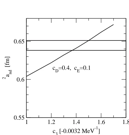
B(4He). Here we are going to use the N2LOL force in con-junction with the AV18 NN interaction, so we have to mod-ify its parametrization since the amount of attraction to be gained is now different (see Table 1). Moreover, the modifi-cation has to be done in such a way that B(3H) and2andare

well reproduced. As an example, in Fig. 5,2and is shown

as a function of the parameter c3 (in units of its original value c3 =0.0032 MeV−1) fixing cD = 0.4,cE =0.1 and

varying c4 in order to reproduce B(3H). With the values

c3=−0.0048 MeV−1, c4=0.0043 MeV−1,2andfall inside

the box and matches the experimental value. In this case, the4_{H binding energy results B(}4_{H)=28.36 MeV.}

5 Polarization observables with the new

parametrizations

In the previous section we have analyzed different parametrizations of the TM’, URIX and N2LOL TNFs de-termined in conjunction with the AV18 NN potential. With the new parametrizations the three quantities under obser-vation, B(3H),2andand B(4He), are well reproduced.

How-ever, some substantial modifications to the first two mod-els were necessary. In the case of the TM’ interaction, we found necessary to include a repulsive term. In the anal-ysis of the URIX interaction, the strength of the repul-sive term resulted to be more than three times larger. In the case of the N2LOL interaction, a minor adjustment of the parameters was necessary. Now we would like to ana-lyze the effects of the new parametrizations in observables that are not correlated to the binding energies or to2and.

Some polarization observables in p₋d scattering have this

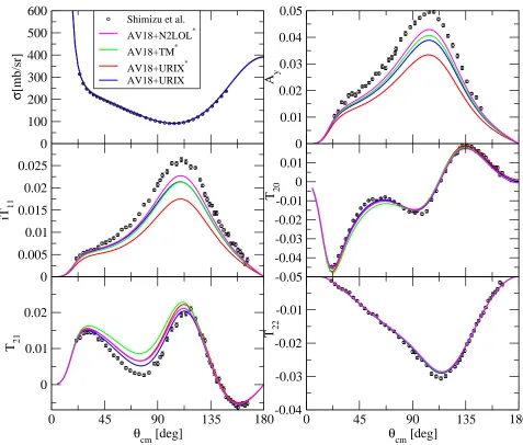
characteristic, in particular the vector and tensor analyzing powers. In Fig. 5, the differential cross section dσ/dΩ, the vector polarization observables Ayand iT11and the tensor polarization observables T20, T21and T22are shown at the laboratory energy Elab=3 MeV, for the different potential

models. As a reference we use the AV18+URIX interac-tion given in the figure as a blue line. In the figure, the other three curves corresponds to particular parametrizations of the models that reproduce 2and and B(3H) and

approxi-mate, as much as possible, B(4He). The parametrizations of the models selected for the figure are the following: the AV18+URIX∗model is defined with APW

2π =−0.0293 MeV, DPW

2π =1 and AR =0.018 MeV. In the AV18+TM∗ model we have used a = −0.87 m−1

-0.05 -0.04 -0.03 -0.02 A PW [MeV]_2π

0.5 1 1.5

D 2

π

PW

-0.05 -0.04 -0.03 -0.02 A PW [MeV]_2π

0.5 0.55 0.6 0.65 0.7

2 a

nd

[fm]

-0.05 -0.04 -0.03 -0.02 A PW [MeV]_2π

28.2 28.3 28.4 28.5 28.6

B(

4 He)

(a) (b) (c)

URIX

AV18+URIX

AV18+URIX

Fig. 4.(a) The relative strength DPW

2π as a function of A

PW

2π. In each point of the curve the triton binding energy and

2_{andare well described.}

(b) Values of2_a

ndfor the seven combinations of the parameters indicated as solid points in panel (a). (c) The corresponding predictions for B(4_{He). The crosses indicate the results using the parameters defined in the URIX model}

d = −3.1657 m−3

π , cE = 1, and Λ = 4mπ. In the AV18+N2LO∗model the parametrization corresponds to

c1 =−0.00081 MeV−1(its original value), c3 =−0.0048 MeV−1, c4 = −0.0043 MeV−1, cD = 0.4 and cE = 0.1.

From the figure we can observe that the models describe equally well the differential cross section and the tensor analyzing powers T20,T22. Differences are observed in the vector analyzing powers Ayand iT11. Taking as a reference the results of the AV18+URIX model, in both cases the AV18+URIX∗_{model produces a noticeable worse} descrip-tion whereas the AV18+N2LOL∗slightly improves the de-scription. The new parametrizations of the TNF models overpredict T21 in all cases, in particular the AV18+TM∗ model.

6 The Kohn Variational Principle in terms

of Integral Relations

Recently two integral relations have been derived from the KVP [22]. It has been shown that starting from the KVP, the tangent of the phase-shift can be expressed in a form of a quotient where both, the numerator and the denomi-nator, are given as two integral relations. Let us first con-sider a two-body system interacting through a short-range potential V(r) at the center of mass energy E in a rela-tive angular momentum state l = 0. The solution of the Schr¨odinger equation in configuration space (m is twice the reduced mass),

(₋~ 2

m∇

2

+V₋E)Ψ(r)=0 , (46)

can be obtained after specifying the corresponding bound-ary conditions. For E>0, with k2_=E/(~2_{/m) and}

assum-1 1.2 1.4 1.6 1.8

c₃ [-0.0032 MeV-1] 0.55

0.6 0.65

2 a

nd

[fm] c_D=0.4, c_E=0.1

Fig. 5.2_{andas a function of the c}

3parameter in the N2LOL model.

ing a short-range potential V,Ψ(r)=φ(r)/√4πand

φ(r_{→ ∞})_−→ √k

"

Asin(kr) kr +B

cos(kr)

kr

#

. (47)

With the above normalization, the solutionΨ verifies the following integral relations:

− ~m2 < Ψ|H−E|F>=B with F=

r

k

4π

sin(kr)

0

100

200

300

400

500

600

σ

[mb/sr]

Shimizu et al. AV18+N2LOL* AV18+TM* AV18+URIX* AV18+URIX

0

0.01

0.02

0.03

0.04

0.05

A

0

0.005

0.01

0.015

0.02

0.025

iT

11

-0.05

-0.04

-0.03

-0.02

-0.01

0

0.01

T

0

45

90

135

180

θ

[deg]

0

0.01

0.02

T

0

45

90

135

180

θ

[deg]

-0.04

-0.03

-0.02

-0.01

T

Fig. 6.Cross section, vector and tensor analyzing powers for p−d scattering at Elab=3 MeV. Experimental points are for Ref. [29]

m

~2 < Ψ|H−E|G>=A with G=

r

k

4π

cos(kr)

kr

tanδ=BA . (48)

Explicitly they are

− m

~2√_k

Z ∞

0

dr sin(kr)V(r)[rφ(r)]=B m

~2√_k

Z _∞

0

dr cos(kr)V(r)[rφ(r)]+φ√(0)

k =A,(49)

where in the last integral we have used the property_∇2_(1/r)= −4πδ(r).

In practical cases the solution of the Schr¨odinger equa-tion is obtained numerically. Then, tanδis extracted from

φ(r) analyzing its behavior outside the range of the poten-tial. The equivalence between the extracted value and that one obtained from the integral relations defines the accu-racy of the numerical computation. A relative difference of the order of 10−7of the two values is usually achieved using standard numerical techniques to solve the diff eren-tial equation and to compute the two one-dimensional inte-grals. To be noticed the short range character of the integral relations. This means that the phase-shift is determined by the internal structure of the wave function.

func-tion ˜G = fregG with the property |G(r˜ = 0)| < ∞ and ˜

G=G outside the interaction region. A possible choice is

˜

G= r

k

4π

cos(kr)

kr (1−e

−γr_{) , (50)}

where the regularization function freg=(1−e−γr) has been introduced withγbeing a non linear parameter which will be discussed below. Values verifying γ > 1/r0, with r0 the range of the potential, could be appropriate. The reg-ularized function ˜G (as well as the irregular function G),

verifies the normalization condition

m

~2

h

<F_|H₋E_|G˜>₋<G˜_|H₋E_|F>i=1 . (51)

Therefore the second integral relation in Eq. (48) remains valid using ˜G in place of G,

m

~2 < Ψ|H−E|G˜ >=A , (52) with the explicit form:

m

~2√_k

Z _∞

0

dr cos(kr)V(r)[rφ(r)]+Iγ=A (53)

where in Iγ all terms depending onγ, introduced by freg, are included. Comparing Eq. (53) to Eq. (49) we identify

Iγ =φ(0)/ √

k.

In the following we demonstrate that the relation tanδ=

B/A, which is an exact relation when the exact wave

func-tionΨis used in Eq. (48), can be considered accurate up to second order when a trial wave function is used, as it has a strict connection with the Kohn variational principle.

The connection of the integral relations with the KVP is straightforward. Defining a trial wave functionΨtas

Ψt=Ψc+AF+B ˜G , (54)

withΨc→0 as r→ ∞, the conditionΨt → AF+B G as

r _{→ ∞}is fulfilled. The KVP states that the second order estimate for tanδis

[tanδ]2nd =tanδ₋m

~2 <(1/A)Ψt|H−E|(1/A)Ψt> . (55) The above functional is stationary with respect to varia-tions onΨcand tanδ. Without loosing generalityΨc can

be expanded in a (square integrable) complete basis

Ψc= X

n

anφn(r) . (56)

The variation of the functional with respect to the linear parameters anand tanδleads to the following equations

< φn|H−E|Ψt>=0

<G˜_|H₋E_|Ψt>=0 . (57)

To obtain the last equation, the normalization relation of Eq. (51) has been used. From these two equations,Ψcand

the first order estimate of the phase shift (tanδ)1st can be

determined. To be noticed that the first equation implies

< Ψc|H−E|Ψt >=0. Furthermore, from the general

rela-tion (m/~2₎h_{< Ψt|H−E|G}˜_>−<G˜_|H−E|Ψt>i_{=A, and}

using the second equation in Eq. (57), the following inte-gral relation results

m

~2 < Ψt|H−E|G˜>=A . (58) Replacing the two relations of Eq.(57) into the func-tional of Eq.(55), a second order estimate of the phase shift is obtained

[tanδ]2nd=(tanδ)1st₋ m

~2 <F|H−E|(1/A)Ψt> . (59) Multiplying Eq. (59) by A one gets

B2nd=B1st₋ m

~2 <F|H−E|Ψt> . (60) On the other hand, a first order estimate for the coefficient

B can be obtained from the general relation

m

~2[<F|H−E|Ψt >−< Ψt|H−E|F >]=B 1st

. (61)

Therefore, replacing Eq.(61) in Eq.(60), a second order in-tegral relation for B is obtained. The above results can be summarized as follow

B2nd=−_~m2 < Ψt|H−E|F>

A= _~m₂ < Ψt|H−E|G˜ >

[tanδ]2nd=B2nd/A . (62) These equations extend the validity of the integral rela-tions, given in Eq.(48) for the exact wave funcrela-tions, to trial wave functions. To be noticed that F,G are solutions of the˜

Schr¨odinger equation in the asymptotic region, therefore (H₋E)F_→0 and (H₋E) ˜G_→0 as the distance between the particles increases. As a consequence the decomposi-tion ofΨtin the three terms of Eq. (54) can be considered

formal since, due to the short-range character of the rela-tion integrals, it is sufficient that the trial wave function be a solution of (H₋E)Ψt=0 in the interaction region,

with-out an explicit indication of its asymptotic behavior. This fact, together with the variational character of the relations allows for a number of applications to be discussed in the next sections.

7 Integral Relations for

A

₌

2

,

3

systems

Applications of the integral relations to systems with A=

2,3 are given. We first consider the following central, s-wave gaussian potential

In the A=2 system, the orthogonal basis

φm=L(2)m(z) exp−(z/2) , (64)

with_Lma (normalized) Laguerre polynomial and z =βr,

beingβa nonlinear parameter, is used to expand the wave function of the system

Ψ0=

M_X−1

m=0

a0_mφm. (65)

The Schr¨odinger equation is transformed to an eigenvalue problem that can be solved for different values of the di-mension M of the basis. The variational principle states that

E0=hΨ0|H|Ψ0i ≥E2B , (66) with the equality obtained for M_{→ ∞}. The nonlinear pa-rameterβcan be fixed to make improve the convergence properties of the basis. In fact, for each value of M there is a value ofβthat minimizes the energy. Increasing M, the minimum of the energy becomes less dependent onβ re-sulting in a plateau. Increasing further the dimension of the basis, the extension of the plateau increases as well, with-out any appreciable improvement in the eigenvalue, indi-cating that the convergence has been reached up to certain accuracy. At each stepΨ0 represents a first order estimate of the bound state exact wave function.

In the proposed example the system has only one bound state. So, with proper values of M andβ, the diagonaliza-tion of H results in one negative eigenvalue E0and M−1 positive eigenvalues Ej( j=1, ....,M−1). The

correspond-ing wave functions

Ψj= M_X−1

m=0

amjφm j=1, ....,M−1 , (67)

are approximate solutions of (H₋Ej)Ψj=0 in the

inter-action region. As r_{→ ∞}they go to zero exponentially and therefore they do not represent a physical scattering state. The negative energy E0 and the first three positive energy eigenvalues (Ej, j=1,3) are shown in Fig. 7 as a function

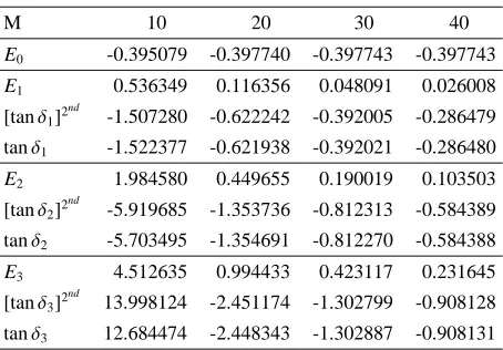
ofβin the case of M=40. We observe the plateau already reached by E0 for the values of βshowed in the figure. We observe also the monotonic behavior of the positive eigenvalues toward zero asβdecreases. The corresponding eigenvectors can be used to compute the integral relations of Eq. (62) and to calculate the second order estimate of the phase-shiftsδjat the specific energies Ej. This

analy-sis is shown in Table 2 in which the non linear parameterβ

of the Laguerre basis has been fixed to 1.2 fm−1_{. In the first} row of the table the ground state energy is given for diff er-ent values of the number M of Laguerre polynomials. The stability of E0at the level of 1 keV is achieved already with

M =20. For a given value of M, Ej, with j=1,2,3, are

the first three positive eigenvalues. The eigenvectors cor-responding to positive energies approximate the scattering states at the specific energies. Since the lowest scattering state appears at zero energy, none of the positive eigenval-ues can reach this value for any finite valeigenval-ues of M. Defining

1 1.5 2 2.5 3

β [fm-1]

-0.5 0 0.5 1 1.5 2

E [MeV]

E₀=-0.397743 MeV

E

1

E₂

E

3

M=40

Fig. 7.The two-nucleon bound state energy E0and the first three

positive eigenvalues Ejas a function ofβin the case of M=40

k2_j = ~m2Ej, the second order estimate for the phase shift at

each energy and at each value of M is obtained as

− m

~2 < Ψj|H−E|Fj>=Bj with Fj= r

kj

4π

sin(kjr)

kjr

m

~2 < Ψj|H−E|G˜j>=Ajwith ˜Gj= freg

r

kj

4π

cos(kjr)

kjr

[tanδj]2

nd

=Bj/Aj. (68)

Table 2.The two-nucleon bound state E0 and the first three

pos-itive eigenvalues Ej ( j = 1,3), as a function of the number of Laguerre polynomials M. The second order estimates, [tanδj]2nd

, obtained applying the integral relations are given in each case and compared to exact results, tanδj.

M 10 20 30 40

E0 -0.395079 -0.397740 -0.397743 -0.397743

E1 0.536349 0.116356 0.048091 0.026008

[tanδ1]2 nd

-1.507280 -0.622242 -0.392005 -0.286479

tanδ1 -1.522377 -0.621938 -0.392021 -0.286480

E2 1.984580 0.449655 0.190019 0.103503

[tanδ2]2 nd

-5.919685 -1.353736 -0.812313 -0.584389

tanδ2 -5.703495 -1.354691 -0.812270 -0.584388

E3 4.512635 0.994433 0.423117 0.231645

[tanδ3]2 nd

13.998124 -2.451174 -1.302799 -0.908128

tanδ3 12.684474 -2.448343 -1.302887 -0.908131

On the other hand, as we are considering the A = 2 system, at each specified energy Ejthe phase shift tanδj

can be obtained by solving the Schr¨odinger equation nu-merically. The two values, [tanδj]2

nd

in the Table 2 at the corresponding energies as a function of M. We observe that, as M increases, the relative diff er-ence between the variational estimate and the exact value reduces, for example at M = 40 is around 10−6. In fact, as M increases, each eigenvector gives a better representa-tion of the exact wave funcrepresenta-tion in the internal region and the second order estimates, [tanδj]2

nd

approach the exact result.

In a different application, the integral relations can be used to calculate the phase-shift of a process in which the two particles interact through a short range potential plus the Coulomb potential, imposing free asymptotic condi-tions to the wave function. As an example we use the same two body potential used in the previous analysis and add the Coulomb potential:

V(r)=−V0exp−(r/r0)2+

e2

r . (69)

For positive energies and l=0, the wave function behaves asymptotically as

Ψ(c)(r_{→ ∞})=AFc(r)+BGc(r) , (70)

with Fc(r),Gc(r) the regular and irregular Coulomb

func-tions, respectively. The phase-shift is tanδc = B/A. The

KVP remains valid when the long range Coulomb potential is considered and its form in terms of the integral relations results:

− ~m2 < Ψ (c)

t |H−E|Fc>=B

m

~2 < Ψ (c)

t |H−E|G˜c>=A

[tanδc]2

nd

= B

A . (71)

with ˜Gc = fregGc andΨt(c) a trial wave function

behav-ing asymptotically asΨ(c)_{. Since (H−E)|F}

c >and (H−

E)_|G˜c>go to zero outside the range of the short range

po-tential, the integrals in Eq. (71) are negligible outside that region. Therefore, for the computation of the phase-shift it is enough to require thatΨ_t(c)verifies (H₋E)Ψ_t(c) =0, inside that region. To exploit this fact, we introduce the following screened potential:

Vsc(r)=−V0exp [−(r/r0)2]+

h

e−(r/rsc)nie 2

r . (72)

For specific values of n and rscit has the property of being

extremely close to the potential V(r) of Eq. (69) for r<r0, with r0the range of the short range potential. The screen-ing factor e−(r/rsc)n _{cuts the Coulomb potential for r >r}

sc.

Using the potential Vscto describe a scattering process, the

wave function behaves asymptotically as

Ψn,rsc(r→ ∞)=AF(r)+BG(r) (73)

with F,G from Eq. (68), since Vscis a short range potential.

Solving the Schr¨odinger equation for this potential, it is possible to obtain the wave functionΨn,rscfor different val-ues of n and rsc. This wave function can be considered as a

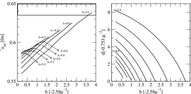
10 20 30 40 50

r_sc [fm] -1

-0.95 -0.9

[tan

δ c

]

2nd

n=1

n=2

n=3

n=4

n=5 n=6 tanδ_c

Fig. 8. The two-nucleon second order estimate [tanδc]2nd

as a function of rscfor different values of n. As a reference the exact value for tanδcis given as a straight line.

trial wave function for the problem in which the Coulomb potential is unscreened. Accordingly it can be used as in-put in Eq. (71) to obtain a second order estimate of the Coulomb phase-shift,

− ~m2 < Ψn,rsc|H−E|Fc>=B

m

~2 < Ψn,rsc|H−E|G˜c>=A [tanδc]2

nd

= B_A (74)

where in H the unscreened Coulomb potential is consid-ered. This estimate depends on n and rscas the wave

func-tion does. In Fig. 8 the second order estimate [tanδc]2

nd is shown as a function of rsc for different values of n. The

straight line is the exact value of tanδc obtained solving

the Schr¨odinger equation. We can observe that for n _≥4 and rsc>30 fm the second order estimate coincides with

the exact results. In this example the integral relations de-rived from the Kohn Variational Principle have been used to extract a phase-shift in presence of the Coulomb poten-tial using wave functions with free asymptotic conditions.

Finally an application of the integral relations to the

A = 3 system is discussed. To this end we give the gen-eralization of the integral relations to the case in which more than one channel is open. The coefficients A and B of Eq. (68) correspond to matrices

Bi j =−

m

~2 < Ψi|H−E|Fj>

Ai j =

m

~2 < Ψi|H−E|Gej>

R2nd =A−1B. (75) with R2nd