Quantitative Analysis of Thoracic Computed Tomography Images

(1)

University of Pennsylvania

ScholarlyCommons

Publicly Accessible Penn Dissertations

1-1-2013

Quantitative Analysis of Thoracic Computed

Tomography Images

Gang Song

University of Pennsylvania, [email protected]

Follow this and additional works at:

http://repository.upenn.edu/edissertations

Part of the

Computer Sciences Commons

This paper is posted at ScholarlyCommons.http://repository.upenn.edu/edissertations/803 For more information, please [email protected].

Recommended Citation

Song, Gang, "Quantitative Analysis of Thoracic Computed Tomography Images" (2013).Publicly Accessible Penn Dissertations. 803.

(2)

Quantitative Analysis of Thoracic Computed Tomography Images

Abstract

Lung disease has risen to the third leading cause of chronic morbidity and mortality in the United States. The diagnosis, differentiation, and classification of the severity of various lung diseases rely on clinical assessment, thoracic imaging using computed tomography (CT), and pulmonary function testing (PFT). While being the reference standard for assessment of the lung's mechanical function, PFT strictly permits a global

measurement of lung physiology.

In contrast, high-resolution image analysis is a powerful tool with the potential for regional as well as global quantification of diseases. Imaging plays an increasingly important role in lung disease diagnosis. Most current pulmonary imaging techniques are used clinically to assess anatomic changes and to provide qualitative or semi-quantitative estimates of disease severity. Although generally effective, radiologic interpretation of CT images is time-consuming, requiring considerable expertise. It is also largely qualitative and prone to inner-observer diagnostic variability. It is therefore desirable to have automated quantitative analysis from imaging modalities.

This dissertation investigates the problem of using thoracic computed tomography images for automatically and quantitatively analyzing and diagnosing lung diseases. We discuss how to complete a holistic automatic pipeline for clinical studies and study its various components. The final goal is to illustrate how to build a complete pipeline using CT images as input and yielding the desired clinical results as output. In the case when a single lung image is provided, we propose an algorithm for segmenting small airways from CT images. When the images at both inspiration and expiration phases are available, we discuss the use of image

registration algorithms to compute lung kinematics, especially focusing on various diffeomorphic transform models. Finally, these image-derived quantitative metrics are analyzed for clinical studies of specific diseases, including differentiation of interstitial lung diseases and chronic obstructive pulmonary diseases, and quantification of small airway air trapping and emphysema. We show that quantitative CT imaging, integrating segmentation, registration, feature computation, feature selection and pattern recognition, can provide better biomarkers for diagnosis and prognosis.

Degree Type

Dissertation

Degree Name

Doctor of Philosophy (PhD)

Graduate Group

Computer and Information Science

First Advisor

James Gee

Second Advisor

(3)

Subject Categories

(4)

QUANTITATIVE ANALYSIS OF THORACIC COMPUTED

TOMOGRAPHY IMAGES

Gang Song

A DISSERTATION

in

Computer and Information Science

Presented to the Faculties of the University of Pennsylvania

in

Partial Fulfillment of the Requirements for the

Degree of Doctor of Philosophy

2013

Supervisor of Dissertation Co-Supervisor of Dissertation

James Gee Jianbo Shi

Associate Professor of Radiologic Science

Associate Professor of Computer and Information Science

Graduate Group Chairperson

Val Tannen, Professor of Computer and Information Science

Dissertation Committee

Jean Gallier, Professor of Computer and Information Science

Warren Gefter, Professor of Radiology

Camillo J. Taylor, Associate Professor of Computer and Information Science

(5)

ACKNOWLEDGEMENT

I would like to express my deepest appreciation and gratitude to my two advisors, James Gee

and Jianbo Shi, for their insightful guidance and patient mentorship, all the way through

my graduate studies at the University of Pennsylvania. I am truly fortunate to have had

the opportunity to work with both of them.

I would like to thank my committee members, Jean Gallier, Warren Gefter, Grace Parraga,

and Camillo J. Taylor, for their invaluable feedback and thought-provoking suggestions to

the completion of this dissertation.

I would like to thank all my collaborators for generously sharing their time and ideas.

Special thanks are extended to Eduardo Mortani Barbosa Jr., Drew Torigian, and Warren,

for providing enormous genuine intellectual advice during our long-time collaboration.

I was lucky to work with a group of wonderful people at PICSL and the CIS Department. I

am sincerely grateful to Brian Avants, Nicholas Tustison, and Paul Yushkevich. They have

inspired my research since the beginning. I would also like to thank Daniel Adler, Elena

Barnardis, Caroline Brun, Phillip Cook, Tessa Sundaram Cook, Sandhitsu Das, Jeffrey

Duda, Yang Alex Liu, Hui Sun, Anh Truong, Hongzhi Wang, Yan Wang, Jue John Wu,

Yuanjie Zheng, and literally every current and past member of PICSL for their tremendous

help and friendship.

I would like to thank my friend, Tingting Sha, for her constant moral support and

end-less encouragement over the past years. I have owned much to her, which goes beyond

words. I would like to thank my amazing parents, Laozhi Song and Chaxiang Wei, for their

unconditional love and dedication. I could not have done this without them.

Finally, I would like to thank and dedicate this dissertation to my grandmother, Yuhua

(6)

ABSTRACT

QUANTITATIVE ANALYSIS OF THORACIC COMPUTED TOMOGRAPHY IMAGES

Gang Song

Jianbo Shi

James Gee

Lung disease has risen to the third leading cause of chronic morbidity and mortality in

the United States. The diagnosis, differentiation, and classification of the severity of

vari-ous lung diseases rely on clinical assessment, thoracic imaging using computed tomography

(CT), and pulmonary function testing (PFT). While being the reference standard for

as-sessment of the lung’s mechanical function, PFT strictly permits a global measurement of

lung physiology.

In contrast, high-resolution image analysis is a powerful tool with the potential for regional

as well as global quantification of diseases. Imaging plays an increasingly important role

in lung disease diagnosis. Most current pulmonary imaging techniques are used clinically

to assess anatomic changes and to provide qualitative or semi-quantitative estimates of

disease severity. Although generally effective, radiologic interpretation of CT images is

time-consuming, requiring considerable expertise. It is also largely qualitative and prone to

inner-observer diagnostic variability. It is therefore desirable to have automated quantitative

analysis from imaging modalities.

This dissertation investigates the problem of using thoracic computed tomography images

for automatically and quantitatively analyzing and diagnosing lung diseases. We discuss

how to complete a holistic automatic pipeline for clinical studies and study its various

com-ponents. The final goal is to illustrate how to build a complete pipeline using CT images

(7)

image is provided, we propose an algorithm for segmenting small airways from CT images.

When the images at both inspiration and expiration phases are available, we discuss the

use of image registration algorithms to compute lung kinematics, especially focusing on

various diffeomorphic transform models. Finally, these image-derived quantitative metrics

are analyzed for clinical studies of specific diseases, including differentiation of interstitial

lung diseases and chronic obstructive pulmonary diseases, and quantification of small

air-way air trapping and emphysema. We show that quantitative CT imaging, integrating

segmentation, registration, feature computation, feature selection and pattern recognition,

(8)

TABLE OF CONTENTS

ACKNOWLEDGEMENT . . . ii

ABSTRACT . . . iii

LIST OF TABLES . . . x

LIST OF ILLUSTRATIONS . . . xviii

CHAPTER 1 Introduction . . . 1

1.1 High Resolution Computed Tomography . . . 2

1.2 Quantitative Information Within HRCT Thoracic Images . . . 3

1.2.1 Within a Single CT image . . . 4

1.2.2 Between a Pair of CT Images . . . 5

1.2.3 Groups of Images . . . 7

1.2.4 Between Imaging and Other Diagnosis Techiniques . . . 7

1.3 Quantitative Analysis of HRCT Pulmonary Images . . . 7

1.3.1 A Holistic Pipeline . . . 8

1.3.2 Automated Image Feature Computation . . . 8

1.3.3 Utilize Image Features for Disease Analysis . . . 10

1.4 Overview of the Dissertation . . . 11

CHAPTER 2 Segmentation of Airway by Removing Paths of Leakage . . . 13

2.1 Introduction . . . 13

2.2 Methods . . . 14

2.2.1 Initial Segmentation Using Speed Function on Adjusted Gradients . 15 2.2.2 Path Candidate Generation from Initial Segmentation . . . 17

(9)

2.3 Results . . . 20

2.4 Discussion . . . 22

CHAPTER 3 Review of Diffeomorphic Deformation Models in Image Registration 24 3.1 Introduction . . . 24

3.2 From Small Deformation to Large Deformation in Image Registration . . . 27

3.2.1 A First Example: Horn-Schunck Optical Flow . . . 28

3.2.2 Demons algorithm . . . 31

3.2.3 Compositive Demons and Inverse Transform . . . 33

3.2.4 Diffeomorphism Group . . . 34

3.2.5 Connection Between Small deformation and Diffeomorphism . . . . 37

3.3 Smooth Vector Fields and Sobolev Gradient . . . 39

3.3.1 Examples of Regularization Terms and Their optimization Operators 39 3.3.2 Sobolev Norm and Sobolev Space . . . 43

3.3.3 Registration in Sobolev Space . . . 44

Sobolev Gradient and Preconditioning . . . 45

3.4 Diffeomorphism with Time-varying Velocity Fields . . . 45

3.4.1 Beg’s LDDMM algorithm . . . 46

3.4.2 Numerical Algorithm of LDDMM . . . 48

3.4.3 Comparison with Horn-Schunck Optical Flow . . . 49

3.4.4 Comparison with Compositive Demons . . . 49

3.5 Diffeomorphism with Stationary Velocity Fields . . . 50

3.5.1 Computation of Exponential Mapping . . . 51

3.5.2 Ashburner’s DARTEL algorithm . . . 51

Comparison with LDDMM . . . 52

3.5.3 Vercauteren’s Diffeomorphic Demons Algorithm . . . 53

Comparison with DARTEL and Compositive Demons . . . 54

3.5.4 Vercauteren’s LogDemons Algorithm . . . 54

(10)

3.6 Conclusion . . . 56

CHAPTER 4 From Affine to Polyaffine Transformation Model . . . 60

4.2 Methods . . . 61

4.2.1 Diffeomorphism in Polyaffine Model . . . 63

4.2.2 Polyaffine Transform Preserving Trajectories . . . 63

4.2.3 Extend Local Region to Trajectory of Local Region . . . 66

4.2.4 Series of Stationary Velocity Field for Trajectory Collision . . . 66

4.3 Implementation . . . 69

4.3.1 Choice of Weight Function . . . 69

4.3.2 Computing Mask Trajectories and Their Collision . . . 72

4.4 Results . . . 73

CHAPTER 5 Diffeomorphic Registration of a Pair of Lung CT Images . . . 76

5.2 Methods . . . 77

5.2.1 Affine Transformation . . . 77

5.2.2 Diffeomorphic Transformations . . . 78

Symmetric Normalization . . . 79

Exponential Mapping . . . 80

5.2.3 Cross Correlation Similarity Metric . . . 81

5.2.4 Optimization Strategy . . . 82

5.3 Results . . . 82

CHAPTER 6 Feature Selection for Characterization of ILD and COPD . . . 89

(11)

6.2.1 PFT Parameters and Image Metrics . . . 93

6.2.2 Feature Selection . . . 94

6.2.3 Classification with SVMs . . . 96

6.2.4 Experiment setup . . . 99

6.3 Results . . . 99

CHAPTER 7 Quantification of Small Airway Air Trapping and Emphysema in Ob-structive Pulmonary Disease . . . 106

7.2 Materials and Methods . . . 108

7.2.1 Patient selection . . . 110

7.2.2 Image acquisition . . . 110

7.2.3 Image analysis . . . 110

7.2.4 Statistical analysis . . . 112

7.3 Results . . . 112

7.5 Conclusion . . . 126

CHAPTER 8 Conclusion . . . 127

(12)

LIST OF TABLES

Table 3.1 Comparison of the parameterization and the regularization terms. For

the operator L, the regularization term is kL · k2_{. Tikhonov}

regular-ization corresponds to Gaussian smoothing. . . 59

Table 5.1 Results using greedy SyN for each scan pair, per category and

over-all. Rankings and final placement are from a total of 34 competing

algorithms. The total running time for each pair is shown on the last

column. . . 83

Table 5.2 Results using exponential mapping for each scan pair, per category and

overall. Rankings and final placement are from a total of 34 competing

algorithms. The total running time for each pair is shown on the last

column. . . 84

Table 6.1 Statistics of ILD patients. . . 91

Table 6.2 Statistics of COPD patients. . . 92

Table 6.3 All 21 PFT values (1st and 3rd rows) and corresponding relevance

values (2nd and 4th rows) to the disease types. . . 93

Table 6.4 Computed image metrics and their relevance to the disease types. G1

denotes the metrics computed from the expiratory images; G2 from

the inspiratory images. Metrics ofG3 are generated by subtractingG1

from G2 . Within each of G1/G2/G3, the metrics are indexed from 1

to 31. The numbers in last three columns are the relevance values to

(13)

Table 6.5 The first 20 selected features from mRMR on both PFT values and

image metrics. Note these features include both PFT values and

im-age metrics. The imim-age metrics includes both the first order statistical

measurements obtainable from the attenuation histogram and other

more sophisticated metrics of texture descriptions. G1: from the

ex-piratory volumes, G2: from the inspiratory volumes,G3: subtracting

G1 from G2 (same as in Table.6.4). . . 103

Table 7.1 Calculated volumes (in ml) and sample standard deviation for all

pa-tients (n=17), subgroup of negligible emphysema (n=7), and subgroup

with moderate/severe emphysema (n=10). . . 112

Table 7.2 Pearson linear correlation coefficients and respective p-values between

key PFT parameters and calculated emphysema and small airway air

(14)

LIST OF ILLUSTRATIONS

Figure 1.1 A representative thoracic HRCT image volume, displayed in 2D slices

of (a) axial, (b) sagittal, and (c) coronal planes. The resolution is

1x1x1mm3. . . 3

Figure 1.2 A visual comparison of CT images of (a) interstitial lung disease and

(b) chronic obstructive pulmonary disease. Note the visually different

texture patterns for the two diseases. . . 5

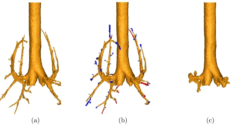
Figure 1.3 An example of airway segmentation using CT image. (a) The

in-put CT image. (b) The segmented airway tree using our method in

Chapter 2. . . 6

Figure 1.4 Deformation between inspiration and expiration. The deformation

field (b) is computed from the CT image at inspiration (a) and the

CT image at expiration (c). A 2D slice of the 3D deformation field is

shown as black-white warped grids. . . 6

Figure 1.5 An example of using run length feature to separate ILD from COPD

on a dataset of 25 patients. The Y axis is the computed value of run

length texture feature. The blue stars on the left of the X axis are

from ILD group and the red stars on the right are from COPD group.

Using this feature computed from CT images, ILD and COPD can

(15)

Figure 2.1 Example of the proposed adjusted image gradients. (a) A region

containing a thin airway (b) Gradients computed as|_OI|. Note that it

has high gradients inside the airway, which prevent fast marching. (c)

Airway segmentation using (b) to compute speed image and MSFM.

(d) Adjusted gradients computed using g(x). Only the gradients in

the bright airway wall are preserved. (e) Airway segmentation using

adjusted gradients in (d) to compute speed image and MSFM. . . . 16

Figure 2.2 Path graph construction. Only the airway tree in the right lung is

shown. (a) Initial segmentationS using fast marching with adjusted

gradients. (b) Distance transformDinsideS with color bar shown on

the right. (c) GraphGusing discretization onD. Nodes{n} are

col-ored by red, green and blue. Each nodenhas the same discretization

value inD0 and belong to the same connected component. (d) Final

segmentation of airway tree using our path segment removal approach. 17

Figure 2.3 Example of the proposed path leakage cost function on a node of

leak-age. Left: shape of the node is similar to airway, but is not part of

airway. First and second rows in the middle: on left) one 2D slice with

the pathnshown in brown; on right) k= 8 sections of the

neighbor-hood ofnin different directions, each sectionNi(n) shown in different

colors. Last row in the middle: bar plots of _|_N1 i(n)|

P

x∈Ni(n)g(x) with

eachishown in corresponding colors. Right: surface rendering of the

k = 8 sections. Location a has an leakage in the upward direction;

however location b is difficult to segment locally. Our proposed cost

S(n) is defined as the minimum of thek= 8 values (the red bar here),

(16)

Figure 2.4 Surface rendering of an example result using the proposed method. (a)

Segmented airway using our approach. (b) Comparison with ground

truth. The blue regions are labeled in ground truth but missing in

our results. The red regions are labeled in our results but missing

in ground truth. The brown regions exist in both ground truth and

our results. (c) Example of the trachea and bronchi region, which is

excluded when computing the rates. . . 21

Figure 3.1 A classical example showing the progress of deforming a half C to a

full C along a diffeomorphism. The deforming grid accompanies each

deformed image. . . 26

Figure 3.2 Fig.1 from [7]. Inversion and composition in a small deformation

setting. The compositions are not identity transform. . . 35

Figure 3.3 Adapted from of Fig.11 from [15]. Each column is a pair of φ1 (first

row) andvtsecond row. Different time points of vt are superimposed

on the same figure. . . 46

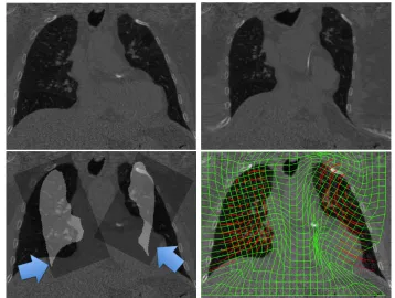
Figure 4.1 Computed tomography images of two lung lobes moving in

differ-ent directions. Top row: images before/after applying the

trans-form. Bottom row: the two local affine transforms and the computed

(17)

Figure 4.2 Polyaffine transform using the previous approach [5]. (a) Two input

affine transforms are shown in red and green. The starting and ending

locations are indicated by the boxes in solid and dashed lines

respec-tively. (b) The input local regions (shown as red and green areas) for

each transform with their velocity plotted inside. (c) Computed

ve-locity field using Eqn. 4.4, interpolated from the input local regions.

(d) The resulting transform. The ending locations of each local region

are plotted as boxes in solid lines at the arrow heads. The solid arrows

(the result) deviate from the dashed arrows (the input), showing that

local transforms are not preserved precisely. . . 64

Figure 4.3 Polyaffine transform using our proposed method. (a) Two input affine

transforms (same as in Fig.4.2(a)) are shown in red and green. The

starting and ending locations are indicated by the boxes in solid and

dashed lines respectively. (b) The trajectories of the input local

re-gions (shown as red and green areas) for each transform with their

velocity plotted inside. (c) Computed velocity field using Eqn. 4.8,

interpolated from the input region trajectories. (d) The resulting

transform. The ending locations of each local region are plotted as

boxes in solid lines at the arrow heads. The solid arrows (the result)

are overlapped with the dashed arrows (the input), showing that local

transforms are preserved precisely. . . 67

Figure 4.4 The trajectories of two local regions overlap. Each arrow represents

an input local transform, plotted in black and red. The boxes at

the arrow tails are the starting locations of each input transform; the

(18)

Figure 4.5 Comparison of the transforms computed using (a,c,e) dist(x, M_i∗), and

(b,d,f) dist(x, ∂M_i∗). (a,b) The transforms are constructed from the

same input, one horizontal translation (green arrow) and one vertical

translation (red arrow). (b) is visually more smooth than (a). (c,d)

The weightsw(x) for the local vertical translation, range in [0,1]. (d)

is more polarized except along boundary ∂M_i∗. (e,f) The resulting

velocity below the green trajectory has an upward vertical component

in (e) but not in (f). Similar effects are seen on the right of the red

trajectory. M_i∗are shown as green and red dotted boundaries in (c,d)

and solid areas in (e,f). . . 70

Figure 4.6 Comparison of our proposed method and the baseline method [5],

using (a) two local translation transforms and (b) two local rotation

transforms. The x-axis corresponds to (a) the translation offset, or

(b) the rotation angle. The y-axis corresponds to the average error

of the resulting transforms in the local affine regions, with standard

deviations plotted as error bars. . . 74

Figure 5.1 The four categories evaluated in the EMPIRE10 challenge: the lung

boundaries, fissures, labeled landmarks and singularities in the

defor-mation field, from [72]. . . 85

Figure 5.2 Examples of good registration results, from two subjects: (a) the fix

subject, (b) the moving subject, (c) the warped moving subject. . . 86

Figure 5.3 Example of bad registration shown in enlarged image region. The

vessels and the fissure in the upper region do not align well. The

remaining lower region, however, has a good registration. . . 86

(19)

Figure 6.2 Examples of SVMs on a synthetic 2D data set. Each data point has its

x and y coordinates as two features. Type I points are marked with red

dots; type II with blue crosses. SVM hyperplanes are shown in green.

Note that Type I points cannot be separated from type II points by

any straight lines. (a) The linear kernel SVM misclassifies several

points, marked with circles. (b) The RBF kernel SVM classifies all

the points with a curve as classification hyperplane. . . 98

Figure 6.3 Relevance (mutual information) of image metrics to different disease

types. The x axis has the image metrics index listed in Table 6.4.

Red bars are for metrics from G1, the expiratory images; blue bars

for G2, the inspiratory images; and green bars for G3, difference of

G1 toG2. . . 99

Figure 6.4 Relevance (mutual information) of PFT values to different disease

types. The x axis lists all the 21 PFT values in Table 6.3. Note that

the range of the y axis is similar to the range from those image metrics

in Fig. 6.3. . . 100

Figure 6.5 Classifying ILD and COPD using the firstn= 1 to 20 selected features

with (a) linear SVM and (b) RBF SVM, using MaxRel or mRMR on

PFT values, image metrics or both PFT and image metrics. For each

curve, the x axis is the number of selected features for training and

testing with SVMs; the y axis is the average error rate from

leave-one-out tests. One subject is excluded when learning SVM parameters

and that subject is used to test the accuracy of the trained SVM. . . 101

Figure 6.6 Receiver operating characteristic curves for using different values to

separate ILD and COPD. The green curve uses FEV1/FVC value.

The red curve uses the RBF SVM scores computed from the first 10

features selected by mRMR. SVMs are trained and tested using the

(20)

Figure 7.1 Illustration of the effectiveness of the registration algorithm. (a)

Representative coronal thoracic HRCT image. (b) Superimposed 3D

lung and central airways segmentation. (c) Coronal subtraction

im-age (inspiration-expiration) prior to registration. Vessel and airway

misalignment is noted. (d) The same subtraction after registration.

Vascular and airway alignment are substantially improved, indicating

the correctness of the registration mapping. Brighter areas indicate

greater difference in attenuation values. . . 109

Figure 7.2 Representative thoracic HRCT images in (a) axial, (b) sagittal, and

(c) coronal planes in subgroup 1 patient with obstructive lung disease

(negligible emphysema). Segmented small airway air trapping shown

in red and segmented emphysema is shown in green in (d) axial, (e)

sagittal, and (f) coronal planes. . . 113

Figure 7.3 Representative thoracic HRCT images in (a) axial, (b) sagittal, and

(c) coronal planes in subgroup 1 patient with obstructive lung disease

(moderate/severe emphysema). Segmented small airway air trapping

shown in red and segmented emphysema is shown in green in (d) axial,

(e) sagittal, and (f) coronal planes. . . 114

Figure 7.4 Computed volumes for each change threshold for the negligible

em-physema subgroup (n = 7 patients). Error bars denote 1 standard

deviation. ATV, small-airway air-trapping volume; EV, emphysema

volume; HU, Hounsfield units; TSLVe, total segmented lung volume

(21)

Figure 7.5 Computed volumes for each change threshold for the moderate or

severe emphysema subgroup (n = 10 patients). Error bars denote

1 standard deviation. ATV, small-airway air-trapping volume; EV,

emphysema volume; HU, Hounsfield units; TSLVe, total segmented

lung volume in expiration; TSLVi, total segmented lung volume in

inspiration. . . 116

Figure 7.6 Pearsons correlations between forced expiratory volume in 1 second

(FEV1)/ forced vital capacity (FVC) and emphysema volume (EV),

small airway air trapping (AT) volume, and total AT volume at each

specific change threshold (5300 Hounsfield units [HU], in 25-HU

in-crements) for subgroup 1 (n = 7 patients). . . 118

Figure 7.7 Pearsons correlations between residual volume (RV) and emphysema

volume (EV), small airway air trapping (AT) volume, and total AT

volume at each specific change threshold (5300 Hounsfield units [HU],

in 25- HU increments) for subgroup 1 (n = 7 patients).. . . 119

Figure 7.8 Pearsons correlations between residual volume (RV) and emphysema

volume (RV), small airway air trapping (AT) volume, and total AT

volume at each specific change threshold (5300 Hounsfield units [HU],

in 25- HU increments) for subgroup 2 (n = 10 patients). . . 120

Figure 7.9 Pearsons correlations between forced expiratory volume in 1 second

(FEV1)/ forced vital capacity (FVC) and emphysema volume (EV),

small airway air trapping (AT) volume, and total AT volume at each

specific change threshold (5300 Hounsfield units [HU], in 25-HU

(22)

CHAPTER 1 Introduction

The lung is the essential respiration organ for human bodies. Its principal function is to

transport oxygen into the bloodstream and release carbon dioxide into the atmosphere. In

general, the lung can be described as an elastic organ and an elaborate network of connecting

airways, vasculature and pulmonary interstitium. Normal lung tissue has a homogeneous

appearance delineated by lobular boundaries, airways and vascular trees. Numerous

pul-monary diseases affect normal lung mechanics by disrupting the material composition of

the lung, impairing the integrity of the lung’s ability to oxygenate the blood effectively.

Lung disease has risen from to one of the major leading causes of chronic morbidity and

mortality in the United States in recent years [117]. According to the American Lung

Association, one in six deaths in the United States can be attributed to lung decease,

and more than 35 million Americans live with chronic lung disease [2]. Identifying and

diagnosing different lung diseases is challenging. The classical ways include pulmonary

function tests (PFT), lung tissue biopsy analysis and imaging tests.

Pulmonary function tests enable clinicians to evaluate an individual’s respiratory status

[40]. It is a noninvasive method of assessing the integrated mechanical function of the lung,

(23)

much air the lung can hold and how quickly the air can move out when a patient exhales.

It currently comprises the reference standard for pulmonary functional assessments.

Lung tissue biopsy analysis is useful when diagnosing interstitial lung disease. A small

amount of lung tissue sample is obtained from a patient’s lungs for a detailed laboratory

analysis. The amount of tissue sample varies from the head of pin to a larger one using an

invasive surgical biopsy.

Imaging test is another clinical diagnosis method. There are various types of imaging

ap-proaches, which include chest X-ray, computed tomography (CT) and gas diffusion imaging.

The objective of this dissertation is to study how to use lung CT images for a quantitative

analysis of various pulmonary diseases.

1.1 High Resolution Computed Tomography

CT imaging provides a noninvasive way to study pulmonary morphology and lung anatomy.

Tissues of different radiation attenuation show distinct values in their CT images. The

values are measured using Hounsfield Units (HU), which ranges from -1024 to +3071. Air,

for example, does not absorb x-rays and has the least radiation attenuation with the value

as -1000HU. Bones, containing calcium, are normally above 200HU. Fatty tissues and blood

are in the range from -100HU to 200HU. Today’s high-resolution CT (HRCT) is able to

achieve near-isotropic 3D resolution on the order of 0.5 mm and to scan the whole lung in

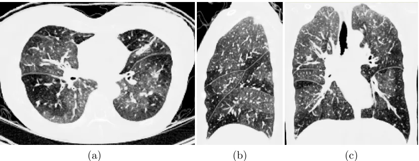
10-25 seconds in expiration or inspiration breath-hold (Fig. 1.1).

Thoracic HRCT of lung imaging is particularly useful for examination of lung parenchyma

in high resolution. It is used to assess a variety of lung pathologies. HRCT image analysis is

a powerful tool with the potential for regional as well as global quantification of pulmonary

diseases.

(24)

non-(a) (b) (c)

Figure 1.1: A representative thoracic HRCT image volume, displayed in 2D slices of (a) axial, (b) sagittal, and (c) coronal planes. The resolution is 1x1x1mm3.

invasive, but it can only provide an overall measurement of pulmonary mechanics. Tissue

biopsy analysis provides accurate information but only around the sampled regions.

On the contrary, imaging provides both a non-invasive and accurate way to analyze the

lung regions. First, CT images provide information on all locations of the lung, not just the

sampled regions in tissue biopsy. Important anatomies like airways and vascular trees are

visible in 3D HRCT images. Additionally, measurements from PFTs are not typically

sen-sitive during early disease development, because affecting a portion of the lung’s functional

ability may not become evident if the rest of the lung is compensating for the dysfunction.

However, imaging can provide direct visualization for clinicians and radiologists to make a

diagnosis on early disease development.

1.2 Quantitative Information Within HRCT Thoracic

Im-ages

There is a wealth of information within HRCT thoracic images for lung disease analysis and

diagnosis. This section discusses the information that is available to extract from different

(25)

1.2.1 Within a Single CT image

To diagnose lung diseases, patients usually undertake scanning at a particular phase of

breathing, for example, at the end of inspiration, or at the end of expiration. There are

various types of information that one can interpret from a single thoracic CT image, e.g.

intensity values, texture information, etc.

The intensity value of each individual voxel is useful in CT images. Different tissues have

different voxel intensities using CT modalities. This fact is useful when differentiating

normal tissue from pathological one. For example, the region with emphysema usually

contains darker voxels. Thus, image thresholding is useful to identify emphysema [79]. By

computing the volume of voxels of intensities below a certain threshold, one can interpret

the severity level of the emphysema.

Texture information also provides distinct visual clues to diagnose lung disease. Although

each individual alveolar is unrecognizable using current CT imaging resolution, the overall

tissue exhibits different visual texture patterns for different lung diseases. For example,

interstitial lung disease (ILD) has certain characteristic texture pattens, when compared

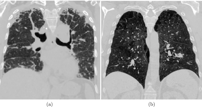
with the CT image of a patient with chronic obstructive pulmonary disease (COPD). Fig.

1.2 shows one image from ILD and one from COPD, where ILD demonstrates a fibrosis

texture pattern, which does not exist in the image of the COPD patient. Such texture

features are crucial to determine the diagnosis and to assess severity of the disease.

Furthermore, important anatomies, like the airway trees, the vascular trees and individual

lobes, are visible from the CT image. An example of the airway tree is shown in Fig. 1.3.

Segmenting the anatomy from CT images helps to identify diseases specifically related to

certain regions, like airway wall attenuation for airway diseases [114]. Using automatic

image segmentation techniques, it is able to have region-specific study by segmenting the

anatomy of interest from the CT image. In other cases, certain anatomies may also be

(26)

(a) (b)

Figure 1.2: A visual comparison of CT images of (a) interstitial lung disease and (b) chronic obstructive pulmonary disease. Note the visually different texture patterns for the two diseases.

1.2.2 Between a Pair of CT Images

The lung is an elastic body, and the respiratory motion is a dynamic procedure. When

multiple CT images scanned at different phases in a breathing cycle are available, the

pulmonary motion can be determined by studying the deformation between images taken

at different phases. A common practice is to take one CT scanning when the patient holds

the breath at the end of inspiration and take the other at the end of expiration. One can

analyze the pulmonary mechanism by computing the deformation field between these two

images. Fig. 1.4 shows an example of the deformation field, computed from the image at

inspiration to the image at expiration.

Once the deformation field is available, certain physical mechanism properties, like Jacobian

or strains, can be further computed to analyze the pulmonary motion. When more than

(27)

(a) (b)

Figure 1.3: An example of airway segmentation using CT image. (a) The input CT image. (b) The segmented airway tree using our method in Chapter 2.

(a) image at inspiration (b) deformation field (c) image at expiration

(28)

1.2.3 Groups of Images

When studying one type of disease, we normally need statistics from a set of images taken

from a group of patient with the same diseases. Another case is longitudinal studies, where

we collect the images of the same patient over multiple time points. These cases lead to

groupwise statistical analysis.

1.2.4 Between Imaging and Other Diagnosis Techiniques

Information within images is valuable and it becomes even more valuable when integrating

together with other clinical diagnoses. For example, studying correlations between image

features and the numbers measured from pulmonary function tests are crucial to research

different diseases. Also, one can investigate the redundancy between imaging diagnosis

and other diagnosis tests by studying whether the information computed from images is

statistically necessary when other diagnosis methods are also available.

1.3 Quantitative Analysis of HRCT Pulmonary Images

While much information exists within thoracic CT images, it requires tremendous effort for

radiologists to observe images, extract information and make diagnosis. Sometimes certain

analysis is very time-consuming or even impossible for humans to complete. For example,

it can take hours or days to segment anatomy structures from a 3D image. This makes it

infeasible to analyze a large-scale dataset. Also, certain tasks are difficult for human vision,

like creating a voxel-wise pulmonary deformation field by aligning two 3D images manually.

Furthermore, with the exponential increase of available imaging data, the required effort

and time will increase explosively.

Therefore, it is desirable to have an automatic computational approach to utilize the

infor-mation from HRCT thoracic images for quantitative analysis and diagnosis. The advantages

(29)

• Reduced human work and errors. This is essential for a reproducible research.

• Quantitative evaluation over qualitative interpretation. For example, rather than

giving an assessment as mild or severe, a continuous number is preferred, which is

more suitable for progressive evaluation.

• Retrospective study on available imaging data. It would be economical to utilize

existing images when new computational methods become available, without the need

of recruiting new patients and taking similar images.

1.3.1 A Holistic Pipeline

In some aspect, the automatic quantitative approach can be viewed as translating the visual

interpretation and reasoning of radiologists to a computational pipeline, or even enhancing

human interpretation by fusing other information in a systematic framework. This is a

challenging task and the main topic of this dissertation.

Quantitative analysis of CT images is not a problem of an isolated module. Instead, it

is more like an integrated pipeline linking different modules using a holistic approach to

integrate various information. In this dissertation, we separate it into two sub-problems:

how to compute various information from images, and how to utilize such information for

disease analysis.

1.3.2 Automated Image Feature Computation

The first sub-problem we are going to address in this dissertation is how to compute

var-ious features from thoracic CT images automatically. As prevvar-iously discussed, there are

multiple types of information which are available from images. Each kind requires a

differ-ent computation method to be extracted. Some of them, like voxel-wise intensity, can be

straightforward as a direct query of CT image arrays. Then the intensity information can

(30)

Other types of information are more challenging to extract. In these cases, more elaborated

algorithms are needed. For example, in the example of differentiating ILD from COPD

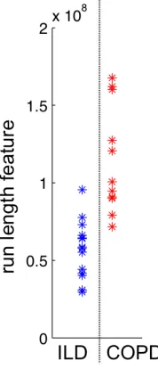
using HRCT images(see Fig. 1.2), one possible way to define the texture is to use run

length feature ([118]), based on computing the voxels of the same intensity level along

different directions. Fig. 1.5 shows that ILD and COPD have separate distinct values

of this feature. Thus, this is an automatic way to replace the visual interpretation from

radiologists to diagnose ILD from COPD.

Figure 1.5: An example of using run length feature to separate ILD from COPD on a dataset of 25 patients. The Y axis is the computed value of run length texture feature. The blue stars on the left of the X axis are from ILD group and the red stars on the right are from COPD group. Using this feature computed from CT images, ILD and COPD can roughly separated.

In the following chapters, we are also going to discuss other types of image features. For

segmenting anatomical structures from a single image, this dissertation will focus on how

to segment the airways in Chapter 2. For computing the deformation field from a pair of

images, we will discuss how to use image registration methods to recover an invertible and

(31)

1.3.3 Utilize Image Features for Disease Analysis

The second sub-problem in this dissertation is how to utilize the features computed from CT

images in the application of disease analysis. Some image features have clinical or physical

interpretation, which can be easily translated using radiologists’ knowledge. For example,

using automatic segmentation of the whole lung region, the volume of segmentation is highly

correlated with the Total Lung Capacity (TLC) measured in the pulmonary function test, as

is discussed in Chapter 7. Also, after aligning a pair of images at inspiration and expiration

phases, the intensity change for each voxel corresponds to the local density change around

the voxel during respiration. These features can be used directly for correlation study or

further analysis.

In other cases, it is not clear whether the computed features are useful for further analysis.

For example, there exist many possible definitions to compute image texture features. It

is desirable to find out which definitions can describe some specific type of disease. In this

case, feature selection can be used in the pipeline to select the most relevant features for

accuracy, or to remove redundant features for simplicity. Furthermore, feature selection can

be applied not only to the image features, but also to other measurements (like pulmonary

function tests) together with image features, to improve diagnosis. We are going to discuss

in detail about how to utilize feature selection to find optimal texture features in Chapter

6.

Besides feature selection, a common practice is to classify different diseases using image

features. This is similar to the case when radiologists make a diagnosis decision based on

the information they observe. We are going to discuss using machine learning methods like

(32)

1.4 Overview of the Dissertation

The topic of this dissertation is to study how to use lung CT images for quantitative analysis

of various pulmonary diseases. The goal is to illustrate how to build a complete pipeline

using CT images as input and the desired clinical results as the output. In the remaining

chapters, we are going to discuss in detail how to compute different types of features from

images and how to utilize these features for disease analysis.

In Chapter 2, we discuss how to segment airway trees from one single thoracic CT image.

We propose a new approach specifically aimed for segmenting thin airway trees.

Different deformation models used in registering two images are reviewed in Chapter 3. We

unify several image registration algorithms in the same framework and compare different

ways to parameterize the deformation model. We specifically discuss the diffeomorphic

deformation models, which are suitable for the physical kinematics of lung respiration.

A new deformation model is proposed in Chapter 4 to balance the parameter complexity

and the model flexibility. Such a new model is suitable as an initial representation of lung

movement for further image registration.

In Chapter 5, we discuss how to adapt the diffeomorphic deformation model in pairwise

lung CT image registration. We demonstrate the accuracy of our registration algorithm by

evaluating them on a public benchmark.

We provide a systematic pipeline in Chapter 6 to identify an optimal set of texture-based

image features in classifying interstitial lung disease and chronic obstructive pulmonary

disease. We demonstrate that image features provide extra information to the measurements

of pulmonary function test.

In Chapter 7, we discuss how to build a pipeline to quantify of small airway trapping and

(33)

trapping can be quantitatively evaluated and automatically located from the CT images.

We conclude with summary and highlight the contributions of this dissertation in Chapter

(34)

CHAPTER 2 Segmentation of Airway by

Removing Paths of Leakage

2.1 Introduction

Segmentation of airway trees from computed tomography images is critical for various

clini-cal applications involving pulmonary diseases. Diameters of the fourth generation airway in

a typical CT image are about two or three voxels wide. The limitation of imaging resolution

and noise lead to the inhomogeneity of image intensities inside airway walls and also the

blurring effects around airway walls. For example, low-dose CT imaging is sometimes

pre-ferred in order to reduce radiation exposure ([105]). These factors make the balance between

detecting over-segmentation and extending thin airway very critical in airway segmentation.

Various algorithms have been proposed in the literature. Schlath¨olter et al used level set

methods for a simultaneous segmentation and tree reconstruction framework [86]. The

authors proposed several heuristic rules to detect leakage in the growing regions. Tschirren

et al proposed to keep an active region of cylinder shape [105]. By tracking the orientation

(35)

multi-threshold approach was adopted in [106] to increase robustness in growing airway

trees. Recent work from Christian et al [14] used gradient vector flow to guide growing

direction. The work of [63] focused on extending thin airway by computing the shortest

paths inside a search sphere from end points in the initial segmentation.

Many of these algorithms have shown successful segmentation of the bronchi and trachea.

However, for the third and higher generations in the airway tree, current segmentation

results still have room for improvement, indicated by a recent evaluation on 15 airway

segmentation algorithms [62].

In this chapter we explore a new approach for airway segmentation. Instead of mixing

airway segmentation and leakage detection at every iteration as in [14, 63], we divide this

problem into a hypothesis generation of thin airway paths and a post processing procedure

of removing leakage path candidates. For the purpose of generating as many hypotheses as

possible, we propose a novel speed function for thin airway. To exclude leakage regions, we

propose a novel cost function defined on the whole path candidate. Such a scheme is more

flexible when evaluating the whole path and can be viewed as complementary to current

region growing methods.

2.2 Methods

Our method includes two steps: path candidate generation and path candidate removal.

In the first step, we generate all initial path candidates in the segmentation using the

fast marching method. A new formulation of adjusted image gradients is proposed to

compute the speed image. Path candidates are then extracted by back tracing in the

arrival time function. Next, those paths which may contain the over-segmentation, or the

leakage regions, are further removed from the initial segmentation using our novel leakage

(36)

2.2.1 Initial Segmentation Using Speed Function on Adjusted Gradients

We use fast marching as the first step to generate the initial airway segmentation. The

arrival time is modeled by the Eikonal equation

|_OT|F = 1, (2.1)

whereF is the speed function of the propagation front andT is the arrival time. Given the

3D image volume I, one common form [86] of the gradient based speed function is

F =e−β|OI|. (2.2)

Here β is a scalar weighting coefficient.

By definition OI usually has high values at the locations close to the boundary of airway,

both inside and outside the airway. Thus fast marching will have a low speed along the

boundary inside airway. For the trachea and bronchi, this is not a practical problem since

the airway boundary takes a small portion in the whole volume. However, for thin airway

(like fourth order airway), where the diameter of the airway is about two voxels wide, the

speedFwould be low along whole thin airway segment and this would prevent fast marching

from successfully extending further (See Fig. 2.1b).

Using |_OI| directly is not suitable for front propagation along thin airway with partial

volume effect. One way to deal with this problem is to interpolate image to a higher

resolution, or to assign a special label for airway boundaries in fast marching. Here we

propose a different solution by adjusting the definition of image gradients. The ideal gradient

for airway segmentation should be defined only on the wall of airway (brighter voxels) rather

(37)

(a) (b) (c) (d) (e)

Figure 2.1: Example of the proposed adjusted image gradients. (a) A region containing a thin airway (b) Gradients computed as |_OI|. Note that it has high gradients inside the airway, which prevent fast marching. (c) Airway segmentation using (b) to compute speed image and MSFM. (d) Adjusted gradients computed using g(x). Only the gradients in the bright airway wall are preserved. (e) Airway segmentation using adjusted gradients in (d) to compute speed image and MSFM.

outside. To formalize this notion, the following modified gradient is proposed:

g(x) =



  

  

|_OI(x)| if|I x+1₂~nx

−I(x)|<|I(x)−I x−1 2~nx

|;

0 otherwise.

(2.3)

~

nx is the unit direction of the gradient: ~nx = _|O_OI_I₍(_xx)₎_| and is measured in voxel units. Note

that this definition is not for leakage detection, but for generating all possible airway

seg-mentation.

With this gradient definition, the corresponding front propagation equation becomes F =

e−βg(x). A seed point x0 in the trachea region is selected as the initial conditionT(x0) = 0.

A comparison of results usingg(x) andOI(x) is shown in Fig.2.1. The fast marching gives

the correct segmentation using the proposedg(x) on this thin airway segment.

Another issue in solving front propagation for thin airway is the choice of connectivities.

Many airway segments are extended along diagonal directions. However, Sethian’s original

fast marching method (FMM, [90]) is not accurate along these directions as it computes

(38)

we applied the multi-stencil fast marching method (MSFM, [46]) to solve the equation in

practice. Compared to FMM, MSFM solves the equation along several predefined stencils

to cover the entire 26 neighboring locations. For those stencils that are not aligned with the

natural coordinate system, the equation is derived using directional derivatives. Details of

MSFM can be found in [46]. Note that a 26-connectivity, which contains connectivity along

diagonal directions in 3D, is especially important for fast marching in thin airway when one

location has no 6-connectivity neighbors in the airway.

2.2.2 Path Candidate Generation from Initial Segmentation

Given the arrival time function T and a threshold t0, the initial segmentation is obtained

as S = {x|T(x) < t0}. S contains both airway tree segments and leakage regions. A nice

property of the functionT is that the propagation path from any given location to the seed

locationx0 can be traced back using the gradient ofT. Our motivation is to cluster voxels

inS into different path segments. In turn, leakage can be detected on voxels in each path

segment as a whole, instead of on each voxel individually.

(a) (b) (c) (d)

Figure 2.2: Path graph construction. Only the airway tree in the right lung is shown. (a) Initial segmentationS using fast marching with adjusted gradients. (b) Distance transform DinsideSwith color bar shown on the right. (c) GraphGusing discretization onD. Nodes

(39)

More formally, a graph G is built to describe the structure of the binary mask S. Each

node in G is a cluster of voxels inS, corresponding to part of the airway or to part of the

leakage. We apply an approach similar to [86] and [47] to get the graph G.

First a distance field,D(x), to the initial seed pointx0 is computed in the domainS. Then

each continuous valueD(x) is discretized into an integerj such that

D0(x) =j, ifjh≤D(x)<(j+ 1)h, (2.4)

in which h is the bin width for discretization. By assigning a node n to one connected

component of the same integer value inD0(x), a graphGis constructed fromS. Neighboring

connected components are connected in the graph. The bin width h controls the shape of

each node in the airway so that a node is roughly a tube-like structure. An example of the

graph construction using discretization is illustrated in Fig.2.2.

The propagation from initial seed pointx0to a voxelx1 inS, denoted asCx1

x0, can be traced

by solving ordinary differential equation

dC(t)

dt =−

OD

|_OD|, withC(t1) =x1 and C(0) =x0. (2.5)

We define the path fromx0 tox1 on the graphG as the series of nodes that intersect with

C(t):

Px1

x0 ={n|n∈G, n∩C

x1

x0 6=∅} (2.6)

2.2.3 Leakage Removal Using Cost Function on Path Nodes

Each path segment node n in G is a candidate for leakage removal. We consider three

properties of the path segment: its volume, its vesselness measurement and how it is

sep-arated from the background in the image. The first two properties have been investigated

(40)

to measure each voxel in n. Those voxels of vesselness smaller than tvessel are removed

from noden. The nodes of a volume greater than a thresholdtvol are also removed. These

two properties make sure that path segmentnis of a tube-like shape, however, it may still

contain leakage areas (see Fig.2.3 for an example).

We propose a novel leakage cost function to estimate how each path node can be separated

from background. For each node n, its medial axis is computed as the segment direction.

The local coordinate system use this direction as z axis of the segment. The surrounding

region of n (obtained from image dilation operation) is then divided into k sections by

different angles uniformly distributed in the x-y plane. Fig.2.3 shows an example ofk= 8

sections in different colors. If the node has leaked into the background from some direction,

the average gradient in that section would be low.

Figure 2.3: Example of the proposed path leakage cost function on a node of leakage. Left: shape of the node is similar to airway, but is not part of airway. First and second rows in the middle: on left) one 2D slice with the pathnshown in brown; on right)k= 8 sections of the neighborhood ofnin different directions, each section Ni(n) shown in different colors. Last

row in the middle: bar plots of _|_N1 i(n)|

P

x∈Ni(n)g(x) with each i shown in corresponding colors. Right: surface rendering of the k = 8 sections. Location a has an leakage in the upward direction; however locationbis difficult to segment locally. Our proposed costS(n) is defined as the minimum of the k = 8 values (the red bar here), which is significantly lower than other bars.

(41)

sections:

S(n) = min

i

1

|Ni(n)|

X

x∈Ni(n)

g(x) (2.7)

where g(x) is the adjusted gradient in section 2.2.1,Ni(n) is the neighborhood of nin the

i-th angle. The nodes of S(n) lower than a threshold tpath are considered as leakage and

are removed from G. The final airway segmentation is the connected component inGthat

contains most remaining nodes.

2.3 Results

The proposed method was applied to extract the airway trees in four canine subjects at

15 months after pulmonary lobe surgery (part of lobes were removed). The images were

acquired under forced inflationary pressure of 30 cm H2O. All images have a slice thickness

of 1.25 mm and in-plane resolution of 0.46×0.46 mm2_{. The airway trees in these volumes}

were semi-supervised extracted and manually modified as the ground truth for evaluation.

In all our experiments, the parameterβ used in computing speed function was set to 0.05.

The initial segmentation threshold t was 200. The distance field D(x) was discretized by

bin width h = 2. The value of h is related to the length of the node in practice. We

tested h from 2 to 4 and got similar results.. We applied the multi-scale strategy when

computing Frangi’s vesselness, using four scaless= 0.5,1,2,3 (see the discussion of scales

in [36]). For each path node n, its surrounding neighborhood was obtained by computing

the dilation of radius= 3 and was further divided to k = 8 sections along the segment

direction. The vesselness threshold tvessel was 30 and the volume thresholdtvol was 1000.

The final segmentation was given by removing all path nodes whose path leakage costS(n)

was lower than 10.

Our method requires a seed point in the trachea region as the initial condition for fast

marching. While such points could be easily manually selected, we further automated the

(42)

roughly aligned with z axis in image volume, we scanned each slice along z axis from the

top and the seed pointx0 was identified as the center of the first detected circle.

(a) (b) (c)

Figure 2.4: Surface rendering of an example result using the proposed method. (a) Seg-mented airway using our approach. (b) Comparison with ground truth. The blue regions are labeled in ground truth but missing in our results. The red regions are labeled in our results but missing in ground truth. The brown regions exist in both ground truth and our results. (c) Example of the trachea and bronchi region, which is excluded when computing the rates.

All final segmentation results S were evaluated against the manually labeled airway trees

Sg. Using| · |to denote the number of voxels in a set, we computed the recall rate as |S∩_|_SS_|g|,

the false alarm rate as |S−Sg|

|S| and the missing rate as |Sg−S|

|Sg| . As trachea and bronchi are

relatively easy to segment using region growing approaches and our main interest was to

extract thin airway, these regions were excluded in computing both S and Sg. Another

reason is that the trachea and bronchi might take up to 95% volume in the whole airway

tree; thus it should be excluded as a huge bias in evaluating thin airway segmentation.

An example of our final segmentation is illustrated in Fig.2.4. Missing regions Sg −S are

colored in blue and false alarm regions S−Sg in red (in Fig.2.4b).

On the four canine subjects, our algorithm got the average recall rate of 96.8% and the

missing rate is 8.2%. Most missing regions are extended from the end segments of 2 to 3

(43)

regions are due to the human label errors. These are not leakage regions in segmentation,

which shows the good performance of our path elimination approach in preventing leakage

while keeping most airway regions.

2.4 Discussion

In this chapter we proposed a new method for extracting airway trees from 3D computed

tomography images. We focused our method on removing leakage regions while still

seg-menting most thin airway. Compared to existing region growing methods, our method had

a unique path removal procedure to exclude potential leakage. A graph of path candidates

was constructed from the arrival time using the fast marching method. The leakage regions

were identified from all path segment candidates using our proposed leakage cost function.

A similar way of checking different directions was proposed in [115]. They used gradients in

different radial directions from one voxel to track vessels. In comparison, our cost function

was defined on the node of a whole path segment for leakage removal. Each node was a

higher level structure, which was more robust to noise and had a more flexible definition.

Furthermore, this was not a linear measurement, which means it could not be represented

as an integration along the path. Thus we did not use Dijkstra’s algorithm, which was used

in [63].

The second contribution in this chapter was that we proposed a form of adjusted gradient in

computing speed image. We also applied multi-stencil fast marching for a 26 connectivity

neighborhood in narrow airway segmentation. We showed that thin airway regions, as

narrow as 1 to 3 voxels wide, could be extracted by our adjusted image gradients and

utilizing the connectivities along diagonal directions in fast marching.

It should be noted that our approach is not contradictory to existing region growing

meth-ods. By separating the leakage detection as a post processing step, our method can take

(44)

one approach can be used as input to the other. For example, the missing rate in our

experiment may be further improved using the method in [63] in the stage of generating

path candidates.

The number of datasets used in the evaluation was limited. A larger evaluation data set is

needed in our future work. Also, we used manual segmentation as our ground truth. An

alternative for constructing the reference is combining results from different algorithms as

in [62]. It would also be interesting to test our algorithm on the output of other algorithms

(45)

CHAPTER 3 Review of Diffeomorphic

Deformation Models in Image

Registration

3.1 Introduction

Image registration is an important medical image analysis technique for computational

research. It generates a transform or a mapping between two given images. Such a mapping

is essential for many medical quantitative research problems. One can construct an anatomy

template by registering a group of images. Various statistics can be defined if images are

registered to the same spatial space. Also, the mapping is useful in building the motion

model for pulmonary and cardiac images. It also helps to discover the longitudinal changes

and quantify the effects of surgical treatments.

Image registration is normally formulated as an optimization problem. An image similarity

function defines how two images are called “similar” after registration. However, this

(46)

assume the optimal transform should be smooth, which is controlled by the regularization

term in the energy function.

Different parameterization of transforms leads to different regularizations. Historically,

transforms with small deformations were first studied as an optical flow problem [53].

Thirion proposed his demons algorithm [101], which was a heuristic approach inspired by

the diffusion process. Due to its practical success, there were theoretical efforts [19] to

justify the demons algorithm later. Small deformations parameterize the transform using

a displacement field, which is analogous to the elasticity of a spring. The performance of

these models usually degrades rapidly for images with large deformation. One important

reason is that the small deformation model does not preserve the topology in the image.

In other words, there is no guarantee regarding the one-to-one mapping property for the

existence of the inverse transform.

Large deformation methods aim to solve this problem by adopting the notion of

diffeo-morphism in image registration. An example was given in Fig. 3.1. A diffeodiffeo-morphism is a

differentiable map with a differentiable inverse, which forms a group structure. It has a solid

mathematical foundation. Unlike small deformation methods, large deformation methods

solve a ”deforming” path of one image transforming into the other. The transform model

was no longer defined on the end point of the transform, but on the entire spatial-temporal

path. This is analogous to tracking motion of the fluid.

Diffeomorphism has been shown as an effective model in computing large deformation

im-age registration. Trouv´e gave some theoretical analysis about the diffeomorphism group in

[104]. Beg et al derived a rigorous model [15] using the velocity fields as parameterization.

To simplify the computation, Ashburner [7] proposed to use a stationary velocity field to

ap-proximate the time-varying velocity field. Especially he introduced a fast numerical method

to compute the derivative in the optimization step. Building on Arsigny’s Log-Euclidean

framework [6], Vercauteren et al adopted the similar idea and extended the classical demons

(47)

approach was formulated more rigorously [110], which worked completely in the log-domain.

Recent improvement by Mansi et al [69] extended the deformation with incompressibility

constraints. Also, interesting work [22] from Chen et al independently proposed another

more flexible way to control both the divergence and the curl of the deformation field.

Figure 3.1: A classical example showing the progress of deforming a half C to a full C along a diffeomorphism. The deforming grid accompanies each deformed image.

One way to understand these diffeomorphic approaches is to study the different forms of

parameterization used in the diffeomorphism model. In this chapter, we focus on four

popular diffeomorphic models: LDDMM from Beg et al [15], DARTEL from Ashburner [7],

diffeomorphic demons [111] and LogDemons [110] from Vercauteren et al.

Our discussion proceeds in two steps. We first unify the general image registration in the

same framework, using the small deformation as examples. We discuss various regularization

approaches applied in these methods and show how they can be unified using the Sobolev

gradient. We explain how the gradient of the image similarity term is mapped to the

transformation space through the regularization term.

After exploiting the shared framework, we focus on discovering the different variants by

contrasting the parameterization of the diffeomorphic transformation models. We compare

the relationship between these algorithms and discuss how they can be converted to each

other by simplifying assumptions or changing optimization schemes, etc. We show that these

large deformation algorithms may be viewed as extensions of the common small deformation

image registration methods.

For a clear comparison, the variant notations used by different authors are unified in this

(48)

background for readers, to aid in a complete understanding of the derivation of the most

important equations. Many techniques commonly used in diffeomorphism can find roots in

the derivation of the small deformation models and the regularization terms.

There are other important problems in diffeomorphic image registration but we could not

cover them in this chapter. A few of them include the image similarity terms, the B-spline

transform model, the second-order optimization schemes, the symmetric scheme and inverse

consistency problem, the numerical methods with Eulerian and Lagrangian coordinates, and

other interesting constraints based on the velocity parameterization.

3.2 From Small Deformation to Large Deformation in Image

Registration

The goal of image registration is to find a viable transform from one image to the other. Such

a transform defines pixel-wise correspondences between two images. To simplify notation,

we assume that any image I discussed here is a scalar function defined on one spatial

domain: I : Ω⊆_Rd_→

R. For example, a 3D image hasd= 3. A transformφis a mapping

between two spatial domains: Ω→Ω. If one transform φis applied to an image I, a new

warped image is generated as the composition of two functionsI◦φ, which is also a function

Ω→_R.

Given an template image I0 (i.e. the fixed image) and an individual image to be warped

I1 (i.e. the moving image), the image registration problem optimizes a transform φ such

that the warped moving imageI1◦φis close to the fixed imageI0 andφis smooth. This is

formulated as minimization of an energy functionE(φ), which usually comprises two parts:

E(φ) =λSS(I0, I1, φ) +λRR(φ), (3.1)

in whichλSandλRare two scalar weights. The first term in the right is an image similarity

(49)

How to choose an appropriate similarity function is a fundamental problem in image

reg-istration, which, however, is not a topic in this chapter. Here we adopt the sum of square

difference (SSD) of two images as the similarity function throughout this chapter, for both

its simplicity and familiarity. One can write SSD as:

S(I0, I1, φ) =kI1◦φ−I0k2. (3.2)

The second part is a transform regularization functionR(φ), which is usually solely defined

on the transform. This term is a prior on the transform smoothness. For some specific

pa-rameterized transformation models, for example, the affine transformation or the B-spline

transformation, the smoothness is implicitly encoded through corresponding

parameteri-zation forms. However, for general non-rigid registration when no other information is

available, the transformφis defined using a deformation vector field u: Ω→R,

φ(x) =x+u(x), x∈Ω. (3.3)

Such a parameterization is simply adding an identity transform with a vector field.

Regu-larization functions are normally defined onuinstead of directly onφ. u(x) is a zero vector

field when φ(x) =x. This form is strongly connected to Hooke’s law about the equilibrium

position of elastic material.

In the rest of this section we particularly elaborate on the mathematical details for the

easy understanding of the derivation details, which is important on the discussion of large

deformation models.

3.2.1 A First Example: Horn-Schunck Optical Flow

There are many choices of regularization terms. One simple model is to constrain first order