The Decline of the Rust Belt: A Dynamic Spatial Equilibrium Analysis

University of Pennsylvania

ScholarlyCommons

Publicly Accessible Penn Dissertations

1-1-2013

The Decline of the Rust Belt: A Dynamic Spatial

Equilibrium Analysis

Chamna Yoon

University of Pennsylvania, [email protected]

Follow this and additional works at:http://repository.upenn.edu/edissertations Part of theEconomics Commons

This paper is posted at ScholarlyCommons.http://repository.upenn.edu/edissertations/724 For more information, please [email protected].

Recommended Citation

Yoon, Chamna, "The Decline of the Rust Belt: A Dynamic Spatial Equilibrium Analysis" (2013).Publicly Accessible Penn Dissertations. 724.

The Decline of the Rust Belt: A Dynamic Spatial Equilibrium Analysis

Abstract

The purpose of this dissertation is to study the causes, welfare effects, and policy implications of the decline of the Rust Belt. I develop a dynamic spatial equilibrium model which consists of a multi-region, multi-sector economy comprised of overlapping generations of heterogeneous individuals. Using several data sets that cover the time period from 1960-2010, I estimate the structural parameters of the model based on a simulated method of moments estimator. The empirical findings suggest that goods-producing firms located in the Rust Belt had a 13 percent relative productivity advantage in 1960 compared to the rest of the U.S., which shrank to approximately 3 percent by the end of the sample period in 2010. As a consequence, a large fraction of the decline of the Rust Belt can be attributed to the reduction in its location-specific advantage in the goods-producing sector. The transition of the U.S. economy to a service sector economy is a less significant factor. The decline of the Rust Belt generated significant differences in welfare between individuals residing in the Rust Belt and those residing in other areas, particularly for the less educated. Policy experiments show that the inequality in welfare can be significantly reduced by subsidizing labor costs in the Rust Belt or reducing mobility costs.

Degree Type

Dissertation

Degree Name

Doctor of Philosophy (PhD)

Graduate Group

Economics

First Advisor

Kenneth I. Wolpin

Subject Categories

THE DECLINE OF THE RUST BELT: A DYNAMIC SPATIAL EQUILIBRIUM

ANALYSIS

Chamna Yoon

A DISSERTATION

in

Economics

Presented to the Faculties of the University of Pennsylvania

in

Partial Fulfillment of the Requirements for the

Degree of Doctor of Philosophy

2013

Supervisor of Dissertation

Kenneth I. Wolpin, Professor of Economics

Graduate Group Chairperson

George J. Mailath, Professor of Economics

Dissertation Committee

Holger Sieg, Professor of Economics

THE DECLINE OF THE RUST BELT:

A DYNAMIC SPATIAL EQUILIBRIUM ANALYSIS

COPYRIGHT

Chamna Yoon

Acknowledgements

I am greatly indebted to my advisors, Kenneth I. Wolpin and Holger Sieg. Through

active discussions and feedback, they motivated me to aim higher and helped me to

become a passionate researcher. I am truly grateful for their continuous support and

inspirations. I would also like to thank my dissertation committee member, Xun Tang

for his guidance and support.

I am also grateful to Aislinn Bohren, Fl´avio Cunha, Francis X. Diebold,

Han-ming Fang, Jeremy Greenwood, Camilo Garcia-Jimeno, Dirk Krueger, Donghoon

Lee, SangMok Lee, Yoonsoo Lee, Iourii Manovskii, Antonio Merlo, Guillermo

Or-do˜nez, ´Aureo de Paula, Andrew Postlewaite, Andrew Shephard, and Petra Todd for

their valuable comments. I thank all of the Penn Economics faculty for being great

examples of dedicated researchers and teachers.

My dissertation was supported in part by the National Science Foundation through

XSEDE resources provided by the XSEDE Science Gateways program (TG-SES120012).

I thank Albert Saiz for generously providing me with satellite-generated land use data.

Last but not least, I would like to thank my wife, Jisoo, and our son, Jonathan,

ABSTRACT

THE DECLINE OF THE RUST BELT: A DYNAMIC SPATIAL EQUILIBRIUM

ANALYSIS

Chamna Yoon

Kenneth I. Wolpin

The purpose of this dissertation is to study the causes, welfare effects, and policy

implications of the decline of the Rust Belt. I develop a dynamic spatial equilibrium

model which consists of a multi-region, multi-sector economy comprised of overlapping

generations of heterogeneous individuals. Using several data sets that cover the time

period from 1960–2010, I estimate the structural parameters of the model based on a

simulated method of moments estimator.

The empirical findings suggest that goods-producing firms located in the Rust

Belt had a 13 percent relative productivity advantage in 1960 compared to the rest of

the U.S., which shrank to approximately 3 percent by the end of the sample period

in 2010. As a consequence, a large fraction of the decline of the Rust Belt can be

attributed to the reduction in its location-specific advantage in the goods-producing

sector. The transition of the U.S. economy to a service sector economy is a less

significant factor. The decline of the Rust Belt generated significant differences in

welfare between individuals residing in the Rust Belt and those residing in other

areas, particularly for the less educated. Policy experiments show that the inequality

in welfare can be significantly reduced by subsidizing labor costs in the Rust Belt or

Contents

Acknowledgements iv

Abstract v

Contents vi

List of Tables viii

List of Figures x

1 Introduction 1

1.1 A Brief History of the Decline of the Rust Belt . . . 7

2 Empirical Analysis 9 2.1 Model . . . 9

2.1.1 Preliminaries . . . 9

2.1.2 Model Specification . . . 10

2.1.3 Solution Algorithm . . . 19

2.2 Estimation Method . . . 22

2.3 Results . . . 26

2.3.1 Parameter Estimates . . . 26

3 Welfare and Policy Analysis 29

3.1 The Decline of the Rust Belt . . . 29

3.2 Welfare Analysis . . . 31

3.3 The Effects of Place-Based Policies . . . 32

3.4 Conclusion . . . 36

3.5 Table and Figures . . . 38

A Additional Model Specifications 63 A.1 Technology . . . 63

A.2 Utility . . . 64

B Weighting Matrix 65

C Data Inputs 67

D Additional Experiment Results 69

List of Tables

3.1 The Rust Belt Shares of Output, Employment, Population, and

Rela-tive Wage . . . 38

3.2 Composition of Workforce and Population . . . 39

3.3 Annual Migration Rate . . . 40

3.4 The Rust Belt Shares of Output, Employment, Population, and Rela-tive Wage . . . 41

3.5 Composition of Workforce and Population . . . 42

3.6 Annual Migration Rate . . . 43

3.7 Production Function (2.1) . . . 44

3.8 Production Shocks (2.2) . . . 44

3.9 Utility Parameters (2.3) . . . 45

3.10 Skill Production Functions (2.5) . . . 46

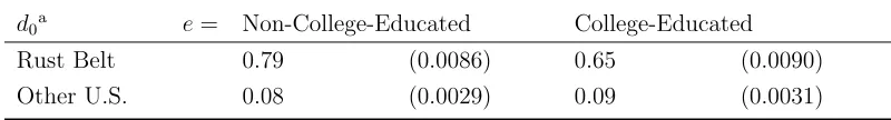
3.11 Type Probabilities: P (θ = 1|d0, e) . . . 46

3.12 Actual and Predicted Rust Belt Shares of Output, Employment, and Population . . . 47

3.13 Actual and Predicted Relative Hourly Wage by Sector . . . 48

3.16 Actual and Predicted Annual Migration Rate by Education Level and

Age . . . 51

3.17 Actual and Predicted Migration Rate by Education Level and Period 52

3.18 Actual and Predicted Mean (log) Housing Expenditure by Education

Level . . . 53

3.19 Actual and Predicted Mean (log) Non-Labor Income by Education Level 54

3.20 The Effect of Sectoral and Regional Technological Changes on Rust

Belt Shares of Output, Employment, and Population . . . 55

3.21 The Effect of Sectoral and Regional Technological Changes on Relative

Wages and the Relative Quality of Local Public Goods . . . 56

3.22 The Difference in Welfare across Regions . . . 57

3.23 Relative (Housing Rental Price Adjusted) Skill Rental Prices, rijet

(pHj_{t )}µ 58

3.24 The Effects of Subsidies on Rust Belt Shares of Output, Employment,

Population, and Relative Wage . . . 59

3.25 The Effects of Subsidies on the Regional Difference in Welfare . . . . 60

3.26 The Effects of Subsidies on Employment Rate, Output, and Welfare . 61

D.1 The Effect of Sectoral and Regional Technological Changes on Rust

Belt Shares of Output and Employment by Sector . . . 70

D.2 The Effect of Sectoral and Regional Technological Changes on Relative

List of Figures

Chapter 1

Introduction

One of the most striking changes in the United States economy over the past 50 years

has been the decline of industrial cities in the Midwest and parts of the Northeast,

an area typically known as the Rust Belt.1 _{The Rust Belt has experienced a relative}

decline in population, wages, and housing rents compared to other areas in the U.S.

In 1960, 27 percent of the U.S. population lived in the Rust Belt. By 2010 the

population of the Rust Belt had decreased to 19 percent. Similarly, in 1960, average

wages and housing rents were higher in the Rust Belt than in other U.S. areas by 10

and 7 percent respectively. By 2010 the wage gap was eliminated and housing rents

in the Rust Belt were 13 percent lower than elsewhere in the states. The purpose of

this dissertation is to study the causes, welfare effects, and policy implications of this

decline.

To understand the causes that led to the decline of the Rust Belt, I develop a new

dynamic spatial general equilibrium model which accounts for changes in comparative

advantages in the production of goods and services, changes in natural,

location-specific advantages, and changes in the supply of skilled workers. There are two

1_{The Rust Belt conventionally includes Illinois, Indiana, Michigan, Ohio, Pennsylvania, and}

regions in the economy, the Rust Belt and the rest of the U.S. In each region, there

are three production sectors: a goods-producing sector, a service sector, and a housing

sector. Goods and services are produced using non-educated labor,

college-educated labor, and capital. Changes over time in the overall productivity of these

sectors in each region are affected by area-specific technological change, sector-biased

aggregate shocks, and changes in magnitude of agglomeration externalities.2

The model is comprised of overlapping generations of heterogeneous individuals

who are born in one of the two regions. Individuals can move between regions, but

face potentially significant mobility costs. Individuals are forward looking and choose

among six discrete alternatives: the two location alternatives, each with three

possi-ble work alternatives (employed in the goods sector, employed in the service sector,

and remaining out of the labor force). Individuals also decide on their consumption

of housing services. In each period, individuals receive a wage offer from each region

and sector, which depends on the region- and sector-specific skill rental price and the

individual’s accumulated specific skill. In equilibrium, a region- and

sector-specific skill rental price is determined by equating the skill price to its marginal

revenue product, evaluated at the aggregate level of skill and capital in that region

and sector. The level of an individual’s skill depends on accumulated work experience

in each sector and on the individual’s level of education. Transitions between sectors

also involve mobility costs which can differ across demographic groups.3 _{I use}

stan-dard, finite-horizon dynamic programing techniques to model the dynamic behavior

of individuals.

2_{The model extends Rosen and Roback’s (1979,1982) static spatial equilibrium to a dynamic}

setting.

3_{My analysis also builds on Topel’s (1986) dynamic general equilibrium of local labor markets}

To close the model, I assume that regional governments provide local public goods

funded through property and income tax revenues. Housing services are produced

using capital and land as inputs. Housing rental prices clear the market for housing

services in each region at each point of time.

I define the dynamic, non-stationary equilibrium for this model. Since equilibria

can only be computed numerically, I develop a new algorithm. Computing

equilib-ria for this model is challenging for a number of reasons. First, I need to solve the

dynamic programming problem of workers accounting for a rich set of state variables

in a non-stationary environment. Second, I need to characterize equilibrium beliefs

that workers hold over the evolution of key state variables. Computing full

ratio-nal expectation equilibria is not feasible. Therefore, I adopt a forecasting rule that

approximates the rational expectations equilibrium (Krusell and Smith, 1998). The

equilibrium beliefs must be self-fullfiling. I adopt an iterative algorithm to determine

the parameters of the beliefs process, extending the procedure developed in Lee and

Wolpin (2006). Third, I need to impose market clearing conditions for a large number

of markets. I show numerically that equilibria exist and can be computed with a high

degree of accuracy.

To obtain a quantitative version of the model, I develop a strategy to estimate

the parameters of the model using a simulated method of moments estimator. I use a

variety of different data sources to construct moments used in the estimation. First,

I have obtained data characterizing employment and wages from the U.S. Current

Population Survey (CPS). Second, I use data on region- and sector-specific output

and capital from the National Income and Product Accounts (NIPA). Third, I

ob-tained access to restricted-use data to calculate sector and regional transition from

the National Longitudinal Survey of Youth 1979 (NLSY79). Finally, I use data on

large vector of moment conditions to identify and estimate the key parameters of the

model.4

Based on the estimated model, I assess the causes of the decline of the Rust Belt.

Relative to a baseline in which there were no economy-wide changes since 1960, I

find that 50 percent of the decline in the Rust Belt’s share of output is due to the

reduction in its location-specific advantage in the goods-producing sector. Relative

to the same baseline, the transition of the U.S. economy to a service sector economy

due to technological change explains 25 percent of the decline. The third important

factor that explains the decline of the Rust Belt is the growth of the share of

college-educated people in the U.S. as a whole.5 Agglomeration externalities and local public

goods provision are endogenous mechanisms that reinforce the decline of the Rust

Belt.

I then investigate the welfare effects of the decline of the Rust Belt. I find that

the average welfare of individuals who resided in the Rust Belt at the age of 20 is

2 to 4 percent lower than that of their counterparts in other areas. The regional

difference in welfare for older individuals who are less mobile is significantly higher;

the gap for them increased by up to 9.7 percent of lifetime welfare. It is also larger

for less-educated individuals, who are estimated to have higher mobility costs.

Given these welfare differences, I consider the impact on the welfare gap of

govern-ment place-based policies, such as wage or migration subsidies. I therefore conduct

a variety of counterfactual policy experiments. Wage subsidy programs are a major

part of the Empowerment Zone program that has been implemented in several

dis-tressed communities in the U.S. over the past 15 years. I find that a 20 percent wage

4_{Estimation is time consuming and is feasible because of super-computing capacity provided by}

the Pittsburgh Supercomputing Center. The gains in computing speed allows me to explore a variety of different model specification.

subsidy for Rust Belt employment can eliminate the welfare gap between the two

areas and increase employment and output in the economy as a whole.6 I also find

that migration subsidies significantly mitigate the welfare gap at a relatively small

cost.

This dissertation is related to several strands of existing literature. There are

cur-rently two major explanations offered in the literature for the decline of the Rust Belt.

First, Blanchard and Katz (1992) and Feyrer, Sacerdote, and Stern (2007) argue that

technological change and economic globalization had a profound impact on regions

oriented towards goods-production, especially on the Rust Belt.7 Second, Glaeser and

Ponzetto (2007) argue that the Rust Belt’s location-specific advantage from easier

ac-cess to waterways and railroads decreased over time. Average freight transportation

costs fell more than 50 percent from 1960 to 2010 due to technological improvements

and the deregulation of the transportation sector (Glaeser and Kohlhase, 2003).8 _I,

however, quantitatively assess the relative importance of several explanations,

includ-ing those aforementioned, which are potentially counteractinclud-ing by placinclud-ing them within

a unified framework.

Recently, Alder, Lagakos, and Ohanian (2012) argue that limited competition in

labor markets and output markets in the Rust Belt is responsible for the region’s

decline. They theoretically show that lack of competition in either labor or output

markets in the Rust Belt can lead to lower investment and productivity of firms in the

region. In contrast to my dissertation, they abstract away from geographic dimensions

6_{Firms in the Empowerment Zone were eligible for a credit of up to 20 percent of the first $15,000}

in wages earned in that year by each employee who lived and worked in the community.

7_{Employment in the goods-producing sector decreased from 42 percent to 22 percent of total}

employment from 1960 to 2010.

8_{Furthermore, water transportation became relatively obsolete; its costs increased and its share}

such as worker’s location choice as well as regional housing markets.

This dissertation is also related to a large literature in urban and labor economics

that analyzes dynamic labor market adjustments and welfare effects of regional shifts

in labor demand. Blanchard and Katz (1992) find substantial population mobility

in response to regional demand shocks. Topel (1986) and Bound and Holzer (2000)

show that less-educated workers are less responsive to these demand changes, and

thus suffer a larger welfare loss from these shocks.There are three key differences

between those studies and my approach. First, I study the labor adjustment across

sectors as well as across regions. Second, I consider the changes in housing rents

and the quality of local public goods as well as in wages. Finally, I explicitly model

individuals’ expectations about future values of these equilibrium objects.

My dissertation is also related to the international trade literature that studies

local labor market outcomes affected by international trade shocks. Autor, Dorn,

and Hanson (2012) and Kovak (2011) study local labor market outcomes from import

competition in the U.S. and Brazil respectively. They find that greater exposure to

import competition substantially decreases employment and wages in the local labor

market. In contrast to these papers where labor is treated as either perfectly mobile

or perfectly immobile, I allow for a costly labor adjustment.

Several recent studies in the labor and urban literature measure the costs of

mi-gration using a dynamic framework (Bishop, 2010; Gemici, 2011; Kennan and Walker,

2011). Migration costs are estimated to be large, amounting to several times the

av-erage annual earning. However, most of these studies focus on the micro-behavior of

migrants, and thus tend to ignore important macroeconomic aspects such as general

equilibrium effects through the labor and housing markets, or aggregate uncertainties

in the economy. I study migration decisions in response to macroeconomic changes

This dissertation also contributes to the growing empirical literature on

place-based policies.9 The literature on state level Enterprise Zones finds mixed evidence

on the effectiveness of these programs at generating jobs.10 On the other hand, Busso,

Gregory, and Kline (2012) find that the federal-level Empowerment Zone program was

able to substantially increased employment and wages for local workers in the zone.

They also find that the efficiency costs of the programs was relatively modest. I study

the possible effects of alternative policies that were not implemented and calculate

their potential welfare costs.

1.1

A Brief History of the Decline of the Rust Belt

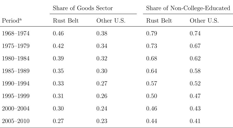
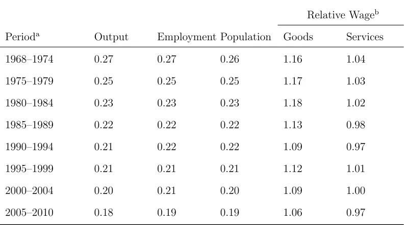
The Rust Belt region has experienced a relative decline in output, employment,

pop-ulation, and wages as seen Table 3.4. Between 1968 and 2010, the Rust Belt’s share of

output decreased by 9 percentage points, from 27 to 18 percent; its share of

employ-ment decreased by 8 percentage points, from 27 percent to 19 percent; and its share

of population decreased by 7 percentage points, from 26 percent to 19 percent.11

The region’s relative drop in wages is most pronounced in the goods sector; the

goods-sector wage gap between the Rust Belt and the rest of the U.S. decreased from

16 percent in 1968 to 6 percent in 2010. The wage gap in the service sector was

smaller than that of goods sector: it decreased from 4 percent to -3 percent over the

same period. Furthermore, the wage drop was not monotonic; there was a relatively

rapid drop during 1975–1994 period. The mean housing rents were higher in the Rust

Belt than in other areas by 7 percent in 1960, but 13 percent lower in 2010.

9_{See Bartik (2002) and Glaeser and Gottlieb (2008) for reviews. See also Moretti (2011) for an}

overview of empirical studies on the place-based policies.

10_{See Busso, Gregory, and Kline (2012) and references therein.}

11_{All nominal figures were converted to 1983 dollars using the gross domestic product (GDP)}

The sector composition of the two regions differed substantially throughout the

period, although similar changes occurred in both regions over time. Table 3.5 shows

the share of goods sector employment in each region.12 The share of goods sector

employment was higher in the Rust Belt by 8 percentage points in 1968–1974 period.

As the U.S. economy shifted from the goods sector to the service sector, the share of

the goods sector decreased in both regions. However, the gap in sector composition

between the two regions also decreased substantially. The share of the

non-college-educated population decreased substantially over the period in both regions (Table

3.5). In 1964–1969 period, the share of the non-college-educated in the Rust Belt was

4 percentage points higher than that of elsewhere in the U.S., but that figure had

increased to 6 percent in 1985–1989 period and then decreased to 3 percent by 2010.

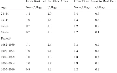
Table 3.6 shows gross flows between regions separately by education level. Younger

and college-educated individuals were more mobile than older and less-educated

in-dividuals. For example, 2.9 percent of college-educated individuals aged 25–34 in

the Rust Belt moved to other areas per year, but that figure was only 0.7 percent for

non-college-educated individuals aged 55–64. The regional mobility rate substantially

decreased over time, especially for college-educated individuals.

12_{The goods sector consists of the mining, construction, and manufacturing industry categories;}

Chapter 2

Empirical Analysis

2.1

Model

2.1.1

Preliminaries

Consider a small open economy with two regions. In each region, there are three

production sectors: the goods-producing sector, the service sector, and the housing

sector. I begin with the assumption that factor and product markets are competitive.

However, these markets differ in their openness. Capital, goods, and service markets

are open, thus the real rental price of capital and real goods and service prices are

exogenous; that is, they are set internationally and taken as given. Labor and housing

markets are not only closed but also regional, and thus their prices are competitively

determined in each region.

On the labor demand side, to capture the efficient allocation of labor and capital

in the equilibrium, it is sufficient to specify production technologies at the

aggre-gate, rather than the firm, level. The setup is that there are eight labor skill types,

two (non-college; college) within each of four regional production sectors (the Rust

U.S.-services). The demand for each skill type is determined by their respective marginal

revenue products. The overall productivity of these sectors in each region can be

affected by region-specific technological change, sector-specific aggregate shocks, and

agglomeration externalities.

At each year between the ages of 25 to 64, individuals have a forecast of how wages

and housing rents will evolve in the future, and choose optimally among six discrete

alternatives: two location alternatives with three work alternatives (goods sector,

ser-vice sector, and out of labor force) within each of the locations. For each period, an

individual receives a wage offer from each region and sector which depends on the

competitively determined region- and sector-specific skill rental price and the

individ-ual’s accumulated sector-specific skill. The level of an individindivid-ual’s skill depends on

accumulated work experience in each sector. Transitions among alternatives involve

a mobility cost which can differ across demographic groups.

Housing services are produced by using capital and land, and are consumed locally.

The housing rental price for each region is determined by the aggregate demand for

and supply of the housing service in that region.

Specific model specification issues are addressed as the details of the model are

presented. Appendix A contains some additional functional form specifications.

2.1.2

Model Specification

Three production sectors are indexed by i ∈ {G: goods;S : service; H : housing}.

Two regions are indexed byj ∈ {1 : the Rust Belt; 2 : the remaining U.S.}.

Technology

The goods-producing sector and the service sector produce output (Y) using

Each sector is also subject to an aggregate productivity shock (ζ). Specifically,

pro-duction of sector i located in region j at time t, valued at the sector’s period t real

price (p), is given by the Cobb-Duglas function,

pij_t Y_tij =pi_tζ_tiβ_tijaij_t F_ti Lij_{N t}, Lij_Ct, K_tij

=z_tiβ_tijaij_t h Lij_{N t}α

i

2t

Lij_Ct1−α

i

2tiα i

1t

K_tij1−α

i

1t

(i=G, S j = 1,2), (2.1)

whereβ_tij is location-specific advantage andaij_t is the agglomeration externality of the

sector i in region j. Following Lucas and Rossi-Hansberg (2002), the agglomeration

externality depends on the aggregate skill density in the region:1

aij_t = L

Gj N t Dj_t

!νi1

LSj_{N t} Dj_t

!ν2i

LGj_Ct D_tj

!ν3i

LSj_Ct D_tj

!ν4i

(i=G, S j = 1,2),

where D_tj is the size of developed land in region j at timet.

Sector-specific real productivity, location-specific advantage, and factor shares

changes are assumed to be time-varying. The sector-specific real productivity is

sub-ject to shocks, zi

t = pitζti, that, evaluated at constant dollars (pit is the real price of

sectorioutput), are assumed to follow a joint first-order vector auto-regressive (VAR)

process in growth rates:2

logzi_t+1−logz_ti = φi₀+ X

k=G,S

φi₁ logzk_t −logz_tk₋₁+i_t+1 (i=G, S), (2.2)

where the innovations are joint normal with the elements of the variance-covariance

matrixσz

ik,i, k =G, S. The location-specific advantageβ ij

t is assumed to be constant

1_{I allow spillovers across sectors.}

2_{I do not distinguish between relative product price changes and sector-specific technological}

up to 1960, then to follow piecewise linear trends with structural breaks at 1975, 1980,

1985, and 1990. The time-varying factor shares, reflecting factor-biased technological

change, are assumed to be constant up to 1960 and then to follow different linear

trends thereafter.

In each region j, housing services are produced using capital and land:3

H_tj =K_tHj αH

Dj_t1−α

H

(j = 1,2).

Demography

The economy consists of overlapping generations of individuals aged 25–64.

Individu-als are initially (at age 25) heterogeneous in terms of their education level,e ∈ {N, C},

and the region where they grew up, d0. In addition, the population consists of nθ

discrete unobservable types (Heckman and Singer, 1984; Keane and Wolpin, 1997) of

individuals who permanently differ in preferences and skill endowments. The

proba-bility distribution of thenθ types is discrete: An individual’s type probability depends

on the place he/she grew up (d0) and education level (e); πθ = P r(θ =i|d0, e) for

i = 1, ..., nθ. Type probabilities are time-varying to the extent that the education

level distribution has changed.

Choice Set

At each age, from a = 25, ...,64, individuals choose among six discrete alternatives:

two location alternatives Ja ∈ {1,2} with three work alternatives Ia ∈ {O, G, S} in

each location.4 They also decide on their consumption level of numeraire and housing

services: ca and ha. I define the following dichotomy variables to denote individual

3_{I ignore labor input for the housing services production function to simplify the analysis, since}

the share of labor input in the housing sector is less than 5%.

decision:

di_a =1{Ia =i}

dj_a =1{Ja =j}

dij_a =1{Ia =i, Ja=j}.

Preferences

The flow utility at each ageafor an individual of education leveleand typeθis given

by

U_aeθ=X

i,j

γ_eθijdij_a +X

j

uq(q_tj)dj_a+uc(ca, ha)−mc

~

da, ~da−1;a, e

, (2.3)

where q_tj is the quality of local public goods in region j, uc(·,·) is the separable

consumption branch of the utility function, and mc(·;a, e) is the psychic cost of

switching regions and/or sectors.

The utility specification allows for differential non-pecuniary benefits associated

with choosing each region-sector, given by γ_eθij for i = G, S, O and j = 1,2. To

capture the strong degree of persistence in the choice of regional alternatives, those

non-pecuniary benefits vary by an individual’s time-invariant type, given by γ_θj for

j = 1,2. I allow age-varying independent and identically distributed (i.i.d.) stochastic

shocks for the non-pecuniary benefit from choosing alternativeO (out of labor force).

Preference shocks are joint normal with elements of the variance-covariance matrix

given by σO

jk,j, k = 1,2. Specifically,

γ_θij =γij +γ_θj (i=G, S j = 1,2)

Individuals have log utilities over local public goods. Specifically,

uq(qj_t) =γqlog(qj_t).

The consumption branch of utility function has a Cobb-Douglas form.5 _Namely,

uc(ca, ha) = (ca)1 −µ

(ha)µ.

Constraints

The individual faces the budget constraint

ca+

X

j=1,2

1 +τ_{P t}j pHj_t hadja =

X

i=G,S

X

j=1,2

1−τ_Itj −τF

wij_at+yet

dij_a, (2.4)

where wij_at is the real wage (earnings) an individual of age a receives from working

in region j and sector i at time t, pHj_t is the housing rental price, τ_{P t}j is the local

property tax, τ_Itj is the local income tax, τF is the federal income tax, and yet is the

education-type-specific non-labor income in period t.

An individual receives a wage offer in each period from each region and in each

sector. I follow the Ben-Porath-Griliches specification of the wage function. Each

sector-region-specific wage offer is the product of a sector-region-specific competitively

determined skill rental prices (r) and the amount of sector-region-specific skill units

possessed by the individual (l). Skill units are produced through work experience (x)

accumulated in each sector, and subject to idiosyncratic i.i.d. shocks. Specifically, a

type-θ individual’s (log) wage offer at ageaand calendar timetin sectoriand region

j is

logwij_a = logr_tij + logl_eθaij (2.5)

= logr_etij +bi_1eθ+ X

k=G,S bik_2exk_a

!bi3

+ij_a.

Sector-specific work experience evolves as xi_a = xi_a−1 +d_ai₋₁, i = G, S. bi_1eθ is the

(sector-specific) education-level-specific skill endowment at age 25 for an individual

of type θ, and the ij

a is an age-varying shock to skill (reflecting, for example, a

health shock). Sector-specific “composite” work experience is a weighted sum of work

experience across all sectors. Thus, in addition to the direct mobility cost associated

with switching employment to a different sector, there is also a loss to the extent

that accumulated work experience in the origin sector produces less composite work

experience in the destination sector, that is, there is a loss of specific skill.

Governments

The regional governments levy a property tax and an income tax based on the

exoge-nously given rates τ_{P t}j and τ_Itj, and spend the revenues to provide local public goods.

The quality of local public goods are determined by the per capita expenditure in

each region (Epple and Sieg, 1999).

Given the linear utility specification, individuals do not have incentive to save,

and thus I assume the federal government levies income τF tax and uses the revenue

ΓF t to invest in domestic capital, Kt+1. Specifically

Kt+1 = (1−δ)Kt+ ΓF t,

Capital and Land Ownership

There are remaining rentals paid to owners of capital and land in this economy. λt

fraction of the total rental income is distributed to college-educated individuals, and

the remaining portion to non-college-educated individuals. Within the two education

groups, individuals own identical diversified portfolios of the domestic capital and

land, and thus have equal shares of domestic capital and land.

Market Clearing and Budget Balance

Each individual alive at time t maximizes the remaining expected discounted present

value of their lifetime utility given their age, subject to (2.3)-(2.5), by choosing among

the six alternatives. The maximized expected lifetime utility of an individual who is

age a at time t is given by

Va(Ωat) = max

{da,ca,ha}

A

X

τ=a

Eρτ−aUτ |Ωat

,

where ρ is the discount factor and Ωat is the information set (or state space) at age

a and time t. The information set consists of current idiosyncratic shocks, years of

education and work experience, current and past skill rental prices, housing rental

prices, non-labor income, the quality of local public goods, and aggregate shocks, as

well as other information used to forecast future prices.

At any time t, agents in the economy form a common forecast of the distribution

of future skill rental prices, housing rental prices, non-labor income, and the quality

of local public goods. Based on that forecast and each agent’s current state, the

alternative that is optimal is chosen. Aggregate skill supplied to each regional sector

is the sum of the skill units of the individuals who choose that alternative. Let Nat

are given by

Lij_{N t} = 64 X a=25 Nat X n=1

lij_natdij_nat1 (enat =N) (i=G, S j = 1,2) (2.6)

Lij_Ct = 64 X a=25 Nat X n=1

lij_natdij_nat1 (enat =C) (i=G, S j = 1,2).

The aggregate supply of capital is perfectly elastic at the current rental price of

capital, and aggregate demand is equal to the sum of demand in the six regional

sectors. Given the static nature of the labor demand side of the model, aggregate

skill demand is determined by equating the marginal revenue product of aggregate skill

for each region and sector to its current (equilibrium) skill rental price. The amount

of capital used in each sector at time t is given by equating the marginal revenue

product of the capital to the exogenous rental price of the capital, rK_t . Specifically,

∂pi tY

ij t zti, L

ij N t, L

ij Ct, K

ij t

∂Lij_{N t} =r

ij

N t (i=G, S j = 1,2)

∂pi tY

ij t zti, L

ij N t, L

ij Ct, K

ij t

∂Lij_Ct =r

ij

Ct (i=G, S j = 1,2) (2.7)

∂pi tY

ij t zti, L

ij N t, L

ij Ct, K

ij t

∂K_tij =r

K

t (i=G, S j = 1,2).

The aggregate housing demand in regionj is the sum of the housing consumptions

of the individuals who choose the region j:

H_tj = 64 X a=25 Nat X n=1

hnatd j

nat (j = 1,2).

Given the exogenous supply of developed land, the aggregate housing supply in region

rental price of the capital, r_tK, so that

H_tj = α

H_pHj t rK

t

! αH

1−αH

Dj_t (j = 1,2). (2.8)

At each time t, the housing demand and supply in each region should be equal.

The regional governments levy a property tax and an income tax based on the

exogenously given rates τ_{P t}j and τ_Itj, and spend the revenues Γj_{P t} and Γj_It to provide

local public goods. The quality of local public goods is determined by the per capita

expenditure of the regional government,

qj_t = Γ

j P t+ Γ

j It

N_tj (j = 1,2), (2.9)

where N_tj is the total population in region j at period t.

Let Y_tK and Y_tD denote the total rents at time t for domestic capital and land

respectively. Specifically,

Y_tK =rK_t Kt

Y_tD = 2

X

j=1

pHj_t H_tj −r_tKK_tHj= 1−αH

2

X

j=1

pHj_t H_tj.

Then, the education-type-specific non-labor income in each period is given by

yCt =

λt YtK +YtD

NCt

yN t =

(1−λt) YtK+YtD

NN t

, (2.10)

where Net is the total number of individuals with education levele in this economy.

equilibrium skill rental prices, housing rental prices, non-labor income, and the quality

of local public goods.

vt=

rG_{N t}1, r_{N t}S1, rG_{N t}2, rS_{N t}2, r_CtG1, rS_Ct1, r_CtG2, rS_Ct2, pH_t 1, pH_t 2, yN t, yCt, qt1, q

2

t

I assume that the solution to (2.7)-(2.10) for the growth rate ofvtcan be approximated

by the function:6

logv_ti₊₁−logvi_t = ηi₀+ 14

X

k=1

ηi_k logv_tk−logv_tk₋₁ (2.11) + ηi₁₅ logz_tG₊₁−logz_tG+η₁₆i logz_tS₊₁−logz_tS.

2.1.3

Solution Algorithm

The solution algorithm is an extension of the method developed in Lee and Wolpin

(2006).7 _{Given the parameters of the model, observed sequences of output in each}

sector, the rental price of capital, the supply of land in each region, and local property

and income tax rates, the algorithm consists of the following steps:

6_{There can be an approximation error because the environment is non-stationary. For example,}

I allow for the growth rates of population and land supply to be non-constant. Therefore, rational expectation would imply that the aggregate state variable process given by (2.11) is also time-varying. Furthermore, I am agnostic as to what individuals know about future technological changes (for example, βij_t and αi_t) or about the future value of other exogenous variables, such as relative product prices, the rental price of capital.

7_{I assume the economy begins in 1860 when I implement the solution algorithm. The age}

1. Choose a set of parameters for the equilibrium aggregate state variable process

(2.11) and for the aggregate shock process (2.2).

2. Solve the optimization problem for each cohort that exists from t= 1 through

t =T. The maximization problem can be cast as a finite horizon dynamic

program-ming problem. The value function can be written as the maximum over

alternative-specific value functions, Vij

a (Ωat), i.e., the expected discounted value of alternative

ij, that satisfies the Bellman equation, specifically,

Va(Ωat) = max i,j

V_aij(Ωat)

V_aij(Ωat) = max ca,ha

U_aij(ca, ha; Ωat) +ρEV Ωa+1,t+1|dijat = 1,Ωat

.

The solution to the optimization problem is in general not analytic. In solving the

model numerically, the solution consists of the values ofEV Ωa+1,t+1|dijat = 1,Ωat

for

all i, j, and elements of Ωat.8 The solution method proceeds by backward recursion.9

3. Let r₁0, p0₁, y0₁, and q₁0 denote the initial guesses for skill rental prices, housing

rental prices, non-labor incomes and the quality of local public goods att= 1. Given

the initial guess and the distribution of state variables for each cohort alive at that

time and between ages 25 and 64, simulate a sample of agents’ chosen alternatives

at t = 1 by drawing from the distribution of the idiosyncratic shocks to preferences

and skills. Given the simulated choices, proceed as a Gauss-Seidel algorithm. First,

compute aggregate skill supplies using relation (2.6), and equate the marginal product

of the capital in each of the four regional-production sectors to the rental price of

8_{I adopt the approximation method developed by Keane and Wolpin (1994) to circumvent the}

curse of dimensionality.

9_{The equilibrium aggregate state variable process (2.11) is assumed to govern the choices made}

capital, which is observed data. Equate the two production functions to the actual

output in the two production sectors. Solve the equations for the optimal capital input

in each region-sector and for the two aggregate shocks, z₁1. Calculate the marginal

product of the skill, at the calculated value of skill, capital, and shocks. Letr1

1 denote

the updated skill rental prices at period one.

Second, calculate rentals for capital and land using updated skill rental prices r1 1.

Compute individual non-labor income y1

1 using the relation (2.10). Third, compute

aggregate housing demand using the updated skill rental prices and non-labor income,

r1₁ and y₁1. Find the housing rental prices p1₁ that equate supply and demand of

housing services. Lastly, calculate regional tax revenues using r1₁, p1₁, and y₁1 and

find the quality of local public goods that satisfies the relation (2.9) to have q1 1. In

general, the updated aggregate state variables, v1

1 = (r11, p11, y11, q11), differ from the

initial guesses.

4. Update the initial guesses for the aggregate state variable to be equal to v1 1.

Repeat step 3 until the sequences of aggregate state variables and aggregate shocks

converge, say to v∗₁ and z∗₁.

5. Guess an initial set of values for the period two aggregate state variables, say

v0 2 =v

∗

1. Repeat steps 3–4 for t= 2 to obtain v

∗

2 and z

∗

2.

6. Repeat step 5 for t = 3, ..., T.

7. Using the calculated series of equilibrium aggregate state variables and

ag-gregate shocks, estimate (2.2), the VAR governing agag-gregate shocks, and (2.11), the

process governing the equilibrium prices.

8. Using these estimates, repeat until the series of aggregate state variables and

2.2

Estimation Method

The model parameters are estimated by simulated method of moments (SMM).10

Specifically, the SMM estimator minimizes a weighted distance measure between

sam-ple aggregated statistics and their simulated analogs. The weights are given by the

inverse of estimated variances of the sample statistics.

The data come from the several sources. The March Current Population Surveys

over the period 1968–2011 and the (restricted-use) National Longitudinal Surveys

1979 youth cohort over the period 1979–1993 provide information on life cycle

em-ployment, location and schooling choices, and wages; various U.S. Censuses from 1960

to 2010 provide data on housing consumption; and National Income and Production

Account (NIPA) provides data on sectoral capital stocks and outputs.11

The simulated aggregate statistics are generated for any given set of parameters

and the derived series of equilibrium prices and aggregate shock by simulating the

behavior of samples of 800 individuals per cohort, starting from cohorts that turned

age 25 in 1929 (and thus would be age 64 in 1968), and ending with cohorts that

turned age 25 in 2010. Therefore, cross-sectional simulated moments contain 32,000

observations. Simulated moments weight each cohort by their representation in the

population of 25 to 64-year-olds.

10_{The model parameters are identified by a combination of functional form and distributional}

assumptions, along with exclusion restrictions. Identification of the wage offer parameters follows from standard selection correction arguments. Utility function parameters are identified because of the existence of variables in the wage function that do not enter the utility function; for example, sector-specific work experience. Identification of production function parameters follows from the existence of valid instruments for input level. Fore example, current and past cohort sizes and renal prices of capital are assumed to be exogenous, and thus are valid instruments. I do not estimate the subjective discount factor. It is instead fixed at 0.95.

11_{I follow the adjustment procedure that is suggested by Lee and Wolpin (2006) when I combine}

The CPS data spans cohorts from 1904 and to 1985 during some period of their

lifetimes between the ages of 25 and 64. CPS data can be used to compute the

choice and wage distributions for those cohorts and ages. However, it does not have

a history of employment choices that would enable the calculation of work experience

because it is primarily a cross-sectional data set. The NLSY79 is a longitudinal data

set that surveys cohorts born from 1957 to 1964 annually from 1979 to 1994 and on a

biennial basis from 1996 to the present. I use the NLSY79 data to calculate aggregate

statistics that represent, or are conditioned on, sector-specific work experience.

The decision period is assumed to be annual in the estimation of the model. To

accommodate the fact that individuals do not necessarily engage in the same activity

over an entire calendar year, the choice variables are defined as follows: an individual

is assigned to the work alternative if he or she worked at least 39 weeks and at least

20 hours per week during the calendar year. When the individual is assigned to the

work category, his or her sector and location is that of the job held during the year

(CPS) or the most recent job (NLSY79). The hourly wage is based on the same job

assignment.

The following is a list of aggregate statistics that are employed in estimation:

1. Career decisions

CPS data

(a) The proportion of individuals choosing each of the six alternatives by year

(1968–2010) and age (25–64).

(b) The proportion of individuals choosing each of the six alternatives by year

and education level (non-college-educated; college-educated).

(c) The proportion of individuals choosing each of the six alternatives by year

(d) The proportion of individuals choosing each of the six alternatives at age

25 by year and location at age 20.

NLSY79 data

(a) The proportion of individuals choosing each of the six alternatives by

ex-perience and education level.

(b) The proportion of individuals choosing each of the six alternatives by

lo-cation at age 20 and edulo-cation level.

2. Wages

CPS data

(a) The mean of the log hourly real wage by region- and sector-categories,

education levels, and year.

(b) The variance of the log hourly real wage by region- and sector-categories,

education levels, and year.12

(c) The mean one-year difference in the log hourly real wage by current and

one-year lagged sector by education level.

NLSY79 data

(a) The mean log hourly real wage by work experience and education level.

(b) The mean log hourly real wage by location at age 20 and education level.

3. Mean non-labor income by year and education levels.

4. Housing expenditures13

(a) The mean of real housing rent by region and year.

(b) The mean of real housing rent by education level and year.

5. Distribution of education level over regions by year and age.

6. Career transitions

CPS data

(a) One-period joint transitions between two location alternatives by year

(1982–2010) and education level.

(b) One-period joint location transitions by age and education level.

(c) One-period joint transitions between two sectors by year.14

(d) One-period joint sectoral and home transitions by age and education level

(matched CPS).

Census data: five-period joint transitions between two location alternatives by

decade (1970–2010) and education level.

NLSY79 data: distribution of years of work experience in each sector.

7. Location- and sector-specific capital and output: by year.15

13_{Following Poterba (1992), I calculate the user cost of housing for a house of market value V}

from the expression,

R= [(1−τy) (i+τj) +ξ]V,

whereτy is the marginal income tax rate,iis the interest rate,τj is the property tax rate, andξis a parameter that captures risk premium and depreciation. I setξ=−0.02 following (Poterba, 1992). I set the marginal tax rate based on tax brackets. For married couples, I impute individual housing expenditures using their wage income share.

14_{A number of years are missing because identifiers that match households between consecutive}

years are not available. The missing transitions are between 1971 and 1972, 1972 and 1973, 1976 and 1977, 1985 and 1986, and 1995 and 1996.

2.3

Results

2.3.1

Parameter Estimates

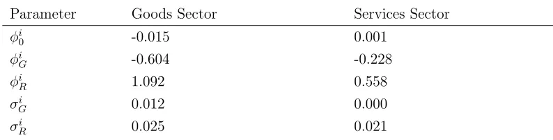
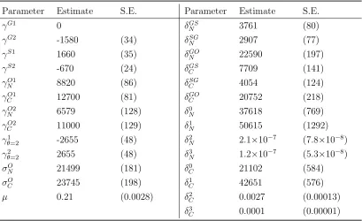
The parameter estimates and their standard errors are shown in Table 3.7–Table

3.11.16 _{I normalize some parameters because skill is not observable, but must be}

inferred from wages. Thus, the constant terms in the skill production functions cannot

be separately identified from the level of skill rental prices. I normalize the constant

term in each sector skill production function for a type 1 person to zero. As a

result, the levels of skill rental prices across sectors are not comparable, although

their changes over time are identified. The non-pecuniary benefits associated with

employment in the goods sector of the Rust Belt are also normalized to zero for a

type 1 person. Therefore, the non-pecuniary benefits of working in the service sector

and consumption values of leisure are relative to this normalization.

The parameters are categorized in the tables as they appear in the model section

according to their equation number. I discuss those that are of particular interest.

Production Function Parameters

Figure 3.5 provides evidence of the significant reduction of the Rust Belt’s

location-specific advantage and the relative decline of goods sector real productivity from 1960

to 2010. The Rust Belt region was 13 percent more productive in producing goods

than other areas in 1960; however, the advantage had fallen to 3 percent in 2010. In

the service sector, the Rust Belt had a small location-specific advantage in 1960, but

had become less productive than other areas in 2010. The combination of product

16_{LetGbe the matrix of derivative of the moments with respect to the model parameters, andS}

price changes and Hicks-neutral technological change led to a relative decline in the

real productivity of the goods sector.

The magnitude of agglomeration externality is small. It explains only one

per-centage point drop in the relative productivity of the goods sector in the Rust Belt.

For the service sector, the agglomeration externality did not play any role.

Utility Parameters

Mobility costs are presented in Table 3.9. The cost of moving between regions within

the same sector is estimated to be significantly larger than moving between sectors

within the same region. For example, for a non-college-educated person aged 26,

the cost of moving between regions is $50,600, but for the same person, the cost of

changing sectors within a region ranges only from $2,907 to $3,761. When changing

regions within a sector, however, the cost is higher for less-educated individuals. For

example, within a sector, the inter regional moving costs are $50,615 and $42,651 for

non-college-educated and college-educated individuals respectively. Conversely, the

cost of changing sectors within a region is higher for college-educated individuals.

For example, the cost of moving from goods sector to the service sector in the same

region is $3,761 and $7,709 for non-college-educated and college-educated individuals

respectively.

Skill Production Functions

Table 3.10 shows the estimates for skill production function parameters. Experience

obtained in a given sector is more transferable to other sectors for college-educated

individuals than for non-college-educated individuals. For example, in the case of

skills gained by non-college-educated individuals in the service sector, the weight on

in the service sector is 0.052. However, in the case of service sector college-educated

skill, the weight on experience gained in the goods sector is 0.047, but the weight on

experience obtained in the service sector is 0.122.

2.3.2

Model Fit

Table 3.12–Table 3.17 present evidence on how well the model fits the data. Table

3.12 compares the Rust Belt shares of output, employment, and population over time

in the actual data to that from the estimated model. The fit for the Rust Belt shares

of output, employment, and population are very close, capturing their decrease over

time. Table 3.13 shows the relative (Rust Belt-to-other U.S. areas) hourly wage by

sector. The fit for the relative hourly wages is also close, although it is slightly

underestimated for the service sector.

The fit of the model with respect to the composition of the workforce and

popu-lation in each region is also close. Table 3.14 shows that the model captures both the

Rust Belt’s higher specialization in the goods sector and the declining goods-sector

share of employment in both areas. As in Table 3.15, the proportion of non-college

educated individuals in each region is also matched very well.

The fit of the model with respect to the extent of state dependence in the choice of

region, in particular, one-period transition rates, is also matched quite well. Table 3.16

shows that the model can fit the fact that young and college-educated individuals are

more mobile than older and less-educated individuals. As in Table 3.17, the estimated

Chapter 3

Welfare and Policy Analysis

3.1

The Decline of the Rust Belt

There are four major exogenous factors in the model that can account for the

rela-tive decline of the Rust Belt: (1) the reduction in the Rust Belt’s location-specific

advantage in the goods sector; (2) the reduction in the Rust Belt’s location-specific

advantage in the service sector; (3) the relative decline of the goods sector real

pro-ductivity in the U.S. economy; and (4) the relative decline of the non-college-educated

population in the U.S. economy. The first three factors are labor demand side

ex-planations for the decline of the Rust Belt. The fourth factor is a labor supply side

change.

To isolate the importance of each factor, I perform the following thought

experi-ment. Suppose the world had stopped changing after 1960 in terms of the four factors

mentioned above. When compared with that world, how would the U.S. economy have

evolved under alternative scenarios in which some of these factors changed as they

did in actuality and others did not, and would those new worlds diverge from what

I consider six counterfactual scenarios. Experiment 1 allows for the reduction of

the Rust Belt’s location-specific advantage in the goods sector. Experiment 2 allows

for the reduction of the Rust Belt’s location-specific advantage in the service sector.

Experiment 3 allows for the real productivity of both sectors to evolve as actually

occurred. Experiment 4 allows for the share of the non-college-educated population in

the U.S. to evolve as it actually did. Experiment 5 simultaneously implements factors

in experiments 1, 2, and 3. And finally, Experiment 6 simultaneously implements

factors in experiments 1, 2, 3, and 4.1

Table 3.20 shows the effects of these four factors on the Rust Belt’s share of

output, employment, and population. I find that each of the four factors accounts

for a substantial part of the relative decline of the Rust Belt. With respect to the

decline of the Rust Belt’s share of output and employment, demand side factors are

important. The results for Experiments 1 and 2 show that about 50 (29) percent of the

decline in the Rust Belt’s share of output can be attributed solely to the reduction in

the Rust Belt’s location-specific advantages in the goods (service) sector. The result

for Experiment 3 shows that the declining real productivity of the goods sector in

U.S. economy explains about 25 percent of the decline.

The labor supply side factor was important for the reduction in the Rust Belt’s

share of the population. My estimate implies that non-college-educated individuals

get higher utility from living in the Rust Belt than the college-educated do. Thus the

reduction in the share of the non-college-educated population generates the relative

decline of the Rust Belt population. Experiment 4 shows that the drop in the share

of the non-college-educated population in the overall U.S. population can account for

1_{For each simulation, I assume that the distribution of entering cohort’s (age 25) initial location}

45 percent of decline in the Rust Belt’s overall share of population.2

Table 3.21 shows the effects of these four factors on the relative (the Rust

Belt-to-other areas) wages and quality of local public goods. As expected, the labor supply

side factor (Experiment 4) cannot account for any part of the relative decline of wages

and the quality of public goods in the Rust Belt. On the other hand, the combined

effect of labor demand side factors (Experiment 5) led to a decrease in the relative

wages and quality of local public goods more than actually occurred.

3.2

Welfare Analysis

In this section, I compute the difference in welfare between individuals in the two

regions in two scenarios: (1) the difference in welfare between individuals who reside

in the Rust Belt at age 20 and those who reside in other areas at age 20; and (2) the

welfare differences for individuals at ages 45–64 with at least 10 years of experience

in the goods sector. The differences are presented in terms of the present value of the

welfare, which are computed over the actual transition path. The welfare differences

are computed for different cohorts and demographic groups.

The first two columns in Table 3.22 show that the welfare losses of the individuals

in the Rust Belt were larger for the non-college-educated population and increased

over time. However, the magnitude of the welfare loss was not large in spite of the fact

that the relative wage of the Rust Belt decreased by more than 10 percentage points

over time. This can be explained by the fact that individuals are relatively mobile

between ages 20 and 25; on average about 8% (22%) of non-college-educated

(college-2_{More precisely, type 1 individuals get higher utility from choosing the Rust Belt than type 2}

educated) individuals moved out of the Rust Belt between ages 20 and 25. The last

two columns in Table 3.22 show that the welfare losses are large for individuals who

are older and have long experiences in goods sector. As expected, the welfare is higher

for individuals in the Rust Belt before 1980 because the older individuals’ remaining

lifetime welfare is mostly determined by the higher goods sector (real) wage in the

Rust Belt (Table 3.23). However, between 2000–2004, the welfare of individuals in the

Rust Belt is lower by 9.7% and 5.8% for non-college-educated and college-educated

individuals respectively.

3.3

The Effects of Place-Based Policies

In this section, I describe the results of simulation experiments designed to examine

how government place-based policies (such as wage or moving subsidies) for the Rust

Belt can influence the dynamic adjustment process, welfare inequality across regions,

and total welfare of the economy.3 _{To satisfy the budget balance need, the costs of}

policies are equally distributed to all the individuals in the economy in the form of a

lump-sum tax.4

First, I consider 10% and 20% wage subsidies for the Rust Belt. The wage subsidy

program is a major part of the Empowerment Zone program that was implemented

in several distressed communities in the U.S. from 1994 to 2009. Firms in the

Em-powerment Zone were eligible for a credit of up to 20% of the first $15,000 in wages

earned in that year by each employee who lived and worked in the community (Busso,

Gregory, and Kline, 2012).

3_{Total welfare of the economy is sum of all the individual utilities in the economy. As I mention}

in Section 3, individuals are owners of labor, domestic capital, and land; therefore, their utilities capture the welfare of capitalists and landlords as well as workers.

4_{More precisely, each individual’s non-labor income decreases to pay the lump-sum tax.}

I also consider a moving subsidy as an alternative policy to mitigate the

wel-fare gap between the regions. Specifically, I subsidize 100% of mobility costs of

non-college-educated (college-educated) 25-year-old individuals who resided in the

Rust Belt at the age 20. The subsidies amount to $37,617 ($21,101) for

non-college-educated (college-non-college-educated) individuals.

Table 3.24 shows the subsidies’ impacts on the Rust Belt’s shares of output,

em-ployment, and population, as well as on the relative wages. The 10% wage subsidy

program reduces the drop in the Rust Belt’s shares of output, employment, and

pop-ulation by approximately 50 percent. However, its impact on the relative wage is

modest. The 20% wage subsidy program enables the Rust Belt to actually increase

its shares of output, employment, and population. In addition, the 20% subsidy

sub-stantially reduces the fall in the relative wage in the Rust Belt. The moving subsidy,

however, exacerbates the decline of the Rust Belt; with it in place, the region’s share

of output, employment, and population decrease further compared to the baseline

case.

Table 3.25 compares the subsidies’ impacts on welfare inequality across regions.

The difference in welfare between the individuals residing in the Rust Belt and those

residing in other areas at age 20 can be reduced about 60%, compared to the baseline

case, by enacting a 10% subsidy. The welfare of the individuals residing in the Rust

Belt actually becomes higher than its counterpart in other areas under the 20% wage

subsidy program. The moving subsidy can also substantially reduce the welfare gap;

the magnitude of its effect is similar to that of 10% wage subsidy.5

Since these policies are implemented at the federal (national) level, it is worthwhile

5_{The moving subsidy increases the non-college-educated (college-educated) individual’s mobility}

to examine their impacts on the entire U.S. economy. Table 3.26 shows the subsidies’

impacts on the employment rate of the economy. The 10% (20%) wage subsidy

increases the employment rate of the Rust Belt by 7.1 (15.9) percentage points. Wages

subsidies also increase the employment rate of the remaining parts of the U.S. This

implies that the wage subsidies generate a net migration flow from the remaining parts

of the U.S. to the Rust Belt; and furthermore, one that is disproportionately composed

of individuals who would have remained out of the labor force in the remaining part of

the U.S. were it not for the wage subsidies that enticed them into the workforce in the

Rust Belt. On the other hand, the moving subsidy decreases the overall employment

rate of the Rust Belt and increases the employment rate of the remaining parts of the

U.S. This implies that the moving subsidy generates a different net migration flow, this

one from the Rust Belt to the remaining parts of the U.S., that is disproportionately

composed of individuals who would have worked in the Rust Belt were it not for

the moving subsidy. The moving subsidy increases the employment rate of the total

economy by reallocating people from the Rust Belt to the remaining part of the U.S.

where overall employment rate is higher.

As seen in Table 3.26, all subsidies increase the total output as the employment

rate increases. The wage subsidy disproportionately increases the output of the goods

sector by increasing the employment rate of the Rust Belt, which has location-specific

advantage in producing goods. On the other hand, the output of the goods sector

decresases under the moving subsidy because the workforce in the Rust Belt migrates

to the remaining parts of the U.S. in which the goods-sector accounts for a relatively

small proportion of production.

Table 3.26 also shows the subsidies’ impacts on the welfare of the economy. The

10% (20%) wage subsidy results in a 0.39% (1.72%) decrease in the total welfare.