DESIGN & FLOW FEATURES OF AXIAL FAN USED IN AN AIR COOLED HEAT EXCHANGER BY EXPERIMENTAL ANALYSIS

273 |

P a g e

DESIGN & FLOW FEATURES OF AXIAL FAN USED

IN AN AIR COOLED HEAT EXCHANGER BY

EXPERIMENTAL ANALYSIS

Arun Patel

, Dr.P.K.Sharma

Prof. Meghna Pathak

M.tech Research Scholar,

Guide & Head,

Co-guide & Assistant Professor,

Mechanical Engineering Department, NRIIST, Bhopal M.P. (India)

ABSTRACT

A heat exchanger is a piece of equipment built for efficient heat transfer from one medium to another. The

media may be separated by a solid wall, so that they never mix, or they may be in direct contact. They are

widely used in space heating, refrigeration, air conditioning, power plants, chemical plants, petrochemical

plants, petroleum refineries, natural gas processing, and sewage treatment. The role of air flow plays vital role

in heat exchanger. Presently heat exchangers use the air flow rate of 5-6 m3/s which gives less efficiency.

Therefore the design of more than 7 m3/s air flow rate in the heat exchanger is done to maintain better

efficiency. The required parameters of air flow fan are air flow, operating temperature, static pressure, Nominal

fan speed, External diameter.

The modification in existing fan was done and desired air flow optimum velocity was achieved 15.23 m/s at

circular duct and 6.675 m/s to archive required parameters.

Keyword: Heat Exchanger, Axial Flow Fans, 1

Tube-Axial Fan, Petroleum Refineries.

I INTRODUCTION

There are two general classifications of fans: the centrifugal or radial flow fan (see ED-2400) and the propeller

or axial flow fan. In the broadest sense, what sets them apart is how the air passes through the impeller. The

propeller or axial flow fan propels the air in an axial direction (Figure 1.1) with a swirling tangential motion

created by the rotating impeller blades. In a centrifugal fan the air enters the impeller axially and is accelerated

by the blades and discharged radially (Figure 1.2).

Figure 1.1 Axial Flow Figure 1.2 Centrifugal Flow

274 |

P a g e

Figure 1.3: Axial flow fan

1.2 Axial Flow Fan Types

Propeller Fans: Sometimes called as the panel fans, propeller fans are the lightest, least expensive and most

commonly used fans. These fans normally consist of a flat frame or housing to be mounted in a wall or in a

partition to exhaust air from a building. This exhausted air has to be replaced by fresh air, coming in through

other openings. If these openings are large enough, the suction pressure needed is small. The propeller fans,

therefore, are designed to operate in the range near free delivery, to move large air volumes against low static

pressures. These fans can be built both direct drive and belt drive (Figure 1.4 and Figure 1.5).

Figure 1.4: Propeller fan with direct drive Figure 1.5: Propeller fan with belt drive

1.2.1Tube-axial Fans

A tube-axial fan is a glorified type of propeller fan with a cylindrical housing about one diameter long,

containing a motor support, a motor and a fan wheel. The motor can be located either on upstream or

downstream of the fan wheel. The fan wheel of a tube-axial fan can be similar to that of a propeller fan. It often

has a medium sized hub diameter,

Figure 1.6: Tube-Axial Fan Figure 1.7: Vane Axial Fan Figure 1.8: Single -Stage Axial Flow Fan

1.3 Performance of Axial Flow Fans

Figure 1.9 shows the shape of a typical pressure versus flow rate curve. Starting from the free delivery, the

pressure value rises to a peak value. This is the good operating range for an axial flow fan. As the air volume

decreases due to increasing restrictions, the axial air velocity decreases as well, resulting in an increased angle

of attack and increased lift coefficients (the phenomena can be understood better in Chapter 2). The increase in

275 |

P a g e

flow results in a decrease in lift coefficient, thus a decrease in pressure occurs.

Figure 1.9: Static Pressure vs. Volume flow rate of an axial fan [24].

1.4 Heat exchangers

Heat exchanger geometry and area are constant by definition in the fixed plant simulations. However, changes

to fluid flow rates will affect the fluid flow regime, equipment operating pressures, and temperature differences

throughout each heat exchanger; which in turn will affect fluid physical properties. Changes in the fluid flow

regime were assumed to have a greater affect on the overall heat transfer coefficient than changes in fluid

properties (viscosity, density, heat capacity, and thermal conductivity).

II LITERATURE REVIEW

Alireza Falahat[ISSN: 2045-7057] et al [2011] In this study an attempt was made to find the best the best angle

of attack and rotational velocity of a flat blade at a fixed hub to tip ratio for a maximum flow coefficient in an

axial fan in a steady and turbulent conditions. In this study the blade angles are varied from 30 to 70 degrees and

the rotational velocity is varied from 50 to 200 rad/sec for a number of blades from 2 to 6, at a fixed hub to tip

ratio. The numerical and experimental results show that, the maximum flow coefficient is achieved at the blade

angle of attack of between 45 to 55 degrees when the number of blades was equal to 4 at most rotational

velocities. The numerical results show that as the rotational velocity increased, the flow coefficient increased but

at very high rotational velocities the flow coefficient remained constant.

Oday I. Abdullah, Josef Schlattmann, et al [2012] In this paper the finite element method has been used to

determine the stresses and deformations of an axial fan blade. Three dimensional, finite element programs have

been developed using eight-node super parametric shell element as a discretization element for the blade

structure. All the formulations and computations are coded in Fortran-77. This work was achieved by modeling

the fan blade as a rotating shell. The investigation covers the effect of centrifugal forces on stresses and

deformations of rotating fan blades. Extensive analysis has been done for various values, speed of rotation,

thickness, skew angle, and the effect of the curvature on the stress and deformation. The numerical results have

shown a good agreement compared with the available investigations using other methods.

Mahajan Vandana N.,Shekhawat Sanjay P et al [2012], In the present paper CFD based investigation has

been reported in order to study the effect of change in speed of fan on velocity, pressure, and mass flow rate of

axial flow fan. It has been observed that there is a significant change in mass flow rate, velocity of rotor and

guide or stator vanes as the speed of fan is varied. As the performance of fan is directly dependent on mass flow

output. So there should be a moderate velocity and pressure profile as all these parameters are co-related. In

276 |

P a g e

software catiav5.

III MATERIAL SELECTION & EXPERIMENTAL SETUP

3.1 Material Selection

In air cooled heat exchanger as they exposed to changing climate condition, the control of the air in the cooler

is relevant. The problem exists in the fan provided in the heat exchanger available in Patel Heat Exchanger, Pvt.

Limited, Govindpura, and Bhopal. It was given the air flow at the rate 5.944 m3/s where as it was required for

efficient cooling at the rate 7 m3/s is above. The design of the fan was done and after proper fabrication the fan

was tested for the desired rate of air flow. The following design considerations were taken into account to

modify the design of the fan.

1. External diameter (d2) of the axial flow fan

2. Internal diameter (d1) of the axial flow fan.

3. Rotational speed (n).

4. Angle of Blade at enter (βº1) & discharge (βº2).

5. No. of Blade (z).

6. Shape & aerofoil section of the Blade.

In the design of single stage axial flow fan, the speed is mainly adapted to the choice of the driving machine,

therefore especially for electrical driver, the speed are generally taken as 1400-1500 rpm. On the basis of

quantities, Ip, n, the peripheral speed, the external fan diameter, the meridional speed and coefficient is

calculated in the following

3.2 Design of axial flow fan (Modified design)

Table 3.1 Requirement of Axial Flow Fan & Input Parameter

We take External Diameter d2 𝑑2= 240𝑉 𝜋2_𝜑𝑛 3

𝜓

Then we find Value φ 𝑑2=_𝜋𝑛60 (2ΔP) / (𝑝)

We find Value this Equation ψ

Take Equation of ψ 𝜓 =_𝜎21_𝛿2

Then we find the value of 𝜎 =2.773 𝛿

And Equation of 𝜑 =_𝜎𝛿1₃

S. No. Require Quantity

1. Air Flow (v) 7 m3/Sec

2. Operating Temperature 30o to 50o

3. Static Pressure 30 mmwg

4. Nominal fan Speed(N) 1450 rpm

5. External Diameter(d2) 0.8m

277 |

P a g e

Then Find Value σ &



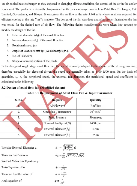
After the value speed coefficient and diameter coefficient is calculated, specific diameter r is read from the

graph given in Figure

Fig. 3.1 Optimum curves with minimal hub ratios for different methods of Installation for

impellers with low characteristics

Specific speed coefficient

The meridional speed is obtained from

𝑐𝑚 = 𝑉

𝜋

4 (𝑑22− 𝑑12) 𝜇2= 𝜋𝑑2𝑛/60

𝜑′_{= 𝑐} 𝑚/𝜇2

Then, 𝑐𝑢=_𝑃𝑢𝜂Δ𝑃

For t/ l, the best value of which range selects the first value are being at the tip of the blade. Thus we have take

number of blade Z

Z= (4π/ 1.5) [sin β2 / {1-(r1/r2)}]

Then obtain value of β2then we take value graph by Eck then we obtain value β1

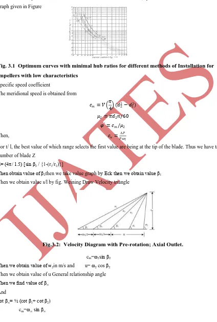
Then we obtain value s/l by fig. Weining Draw Velocity triangle

Fig.3.2: Velocity Diagram with Pre-rotation; Axial Outlet.

cm=ω2sin β2

Then we obtain value of ѡ2in m/s and u= ω2 cos β2

Then we obtain value of u General relationship angle

Then we find value of β∞

And

cot β∞= ½ (cot β1+ cot β2)

278 |

P a g e

Fig.3.3: Distance of Tip and Length of Chord

We find the value of ω∞ v∞ / 2 = ( β2 - β1)/2 βm=(β1+ β2)/2

And value of t/l

Then we take value of by graph t=l cos βm then take l

And we take a value of µ

And (1-µ)/µ = value of this equation

And Value V= (v∞/2){ (1-µ)/µ}

We obtain value v β1´= β1´- v

β2´= β2- v

∆ β=∆ β1(l/t)2 according to Weining graph determining the increase of angle by profiling s, profile thickness , l

chord length

∆ β= value of this equation

We take value of

βm+ ∆ β= value of this equation

3.3 Calculation of Axial Flow Fan

We take External Diameter d2 =0.795 𝑑2= 240𝑉 𝜋2_𝜑𝑛 3

Then we find Value φ 0.795 = 2 _𝜋2𝜑240×7_×1450

Then we find Value φ = 0.22

𝑑2= 60

𝜋𝑛 (2ΔP) / (𝜓𝑝)

0.795 = 60

𝜋 × 1450 2 × 30 / (𝜓 × 1/8)

We find Value this Equation ψ =0.130 Take Equation of ψ

𝜓 = 1

𝜎2_𝛿2

0.130 = 1

𝜎2_𝛿2

Then we find the value of







2

.

773

279 |

P a g e

𝜑 = 1

𝜎𝛿2

0.22 = 1

𝜎𝛿2 Equating both value ψ and ϕ

Then Find Value σ =2.16 & δ=1.28

After the value speed coefficient and diameter coefficient read from the graph given in Figure by Eck

Specific speed coefficient

₄

)

3

/

(

379

.

0

n

V

H





d2=795 mm, & d1= 795 × 28 = 225 mm, η =73%

The meridional speed is obtained from cm=V/(π/4



d

d



2

1

2

2



cm = 15.122 m/sec u2 = πd2n / 60

u2 = 60.73 m/sec

φ’= cm /u2

φ’= 0.24 Then,



pu

p

c





u

c



328

.

76

For t/ l, the best value of which range selects the first value are being at the tip of the blade. Thus we have take

number of blade Z =9.

Z= (4π/ 1.5) [sin β2 /{1-(r1/r2)}]

Then find value β2 = 50.54° ͌ 50°

Then we take fig. blade pitch according to Zweifel

Fig.3.4: Blade Cascades with Optimum Pitch According to Zweifel.

Take according to Zwifel β1= 30°

280 |

P a g e

Fig.3.5: Velocity Diagram with Pre- Rotation; Axial Outlet.

cm=ω2sin β2 ω2 = 19.74 m/sec Then we obtain value of ѡ2 and

u= ω2 cos β2

Then we obtain value of General relationship angle Then we find value of And u =12.68 m/s

cot β∞= ½ (cot β1+ cot β2)

β∞=37.87°

cm=ω∞ sin β∞ ω∞=24.63 m/s

v∞ / 2 = ( β2 - β1)/2=10° βm=(β1+

β2)/2=40°

And value of t/l

Then we take value of by graph

Fig.3.6: A Graph Between Distance of Tip And Length Of Chord

t=l cos βm then take l = 0.085 m

And we take a value of µ = 0.61

And (1-µ)/µ =.0639

And Value V = (V∞/2) { (1-µ)/µ}

V = 6.393

β1´= β1´- V

β1´=23.607°

β2´= β2- V

β2´=56.393

∆ β=∆ β1(l/t)2 according to Weining graph determining the increase of angle by profiling s, profile thickness , l

281 |

P a g e

We take value of βm+ ∆ β=42.39°

3.4 Design Data of Impeller of Existing Fan and Modified Fan

Table3.2: Design data of the fan

Parameter Value of Existing Value of Modified

Design Design

d2 775 mm 795 mm

d1 230mm 225 mm

β1° 25 30

β2° 45 50

L 85mm 85 mm

µ 0.54 0.61

ν 8.51 6.393

0.130 0.130

0.22 0.22

Cm 16.13 15.32

2.16 2.16

z 9 9

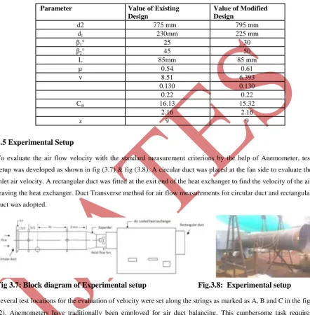
3.5 Experimental Setup

To evaluate the air flow velocity with the standard measurement criterions by the help of Anemometer, test

setup was developed as shown in fig (3.7) & fig (3.8). A circular duct was placed at the fan side to evaluate the

inlet air velocity. A rectangular duct was fitted at the exit end of the heat exchanger to find the velocity of the air

leaving the heat exchanger. Duct Transverse method for air flow measurements for circular duct and rectangular

duct was adopted.

Fig 3.7: Block diagram of Experimental setup

Fig.3.8: Experimental setup

Several test locations for the evaluation of velocity were set along the strings as marked as A, B and C in the fig.

(2). Anemometers have traditionally been employed for air duct balancing. This cumbersome task requires

performing a traverse of the opening, measuring and manually recording the velocity

IV RESULT AND DISCUSSION

The fan of heat exchanger was designed and with modified dimension, the fan was fabricated and installed

in heat exchanger. The modified fan was tested and the details of testing as given below:-

4.1 Testing of fan velocity at different string A, B and C.

The experimental set up was developed to test the air flow velocity of the both the type of duct is circular

282 |

P a g e

efficiency and statistically. The observation of three string A, B and C of air flow velocity have taken are

presented in table no. 4.1

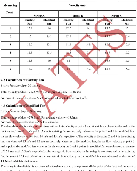
Table 4.1: Air Flow Measurement On The Face Of the Duct By Duct Transverse Method For

Circular Duct.

Measuring Velocity (m/s)

Point

String A String B String C

Existing Modified Existing Modified Existing Modified

Fan Fan Fan Fan Fan Fan

1 12.1 14 12.2 14 13.2 15

2 13 16.2 12.6 15.3 13.5 16.4

3 12.5 15.1 11.6 14.8 12.3 15.6

4 12.8 15.5 12.4 15.1 12.5 15.2

5 12.8 16 12 15 14.5 16.5

6 11.2 15 11 13.2 13.2 15.2

4.2 Calculation of Existing Fan

Statics Pressure (Δp)= 20 mmwg

Total velocity of duct =212.5.9m/s For average velocity =11.82 m/s

Air flow of the circular duct= A V F Where F=1 = 5.944 m3/s Say 6 m3/s

4.3 Calculation of Modified Fan

Statics Pressure (Δp) = 20 mmwg

Total velocity of duct =278.3 m/s For average velocity =15.5m/s

Air flow of the circular duct = A V F = 7.69m3/s

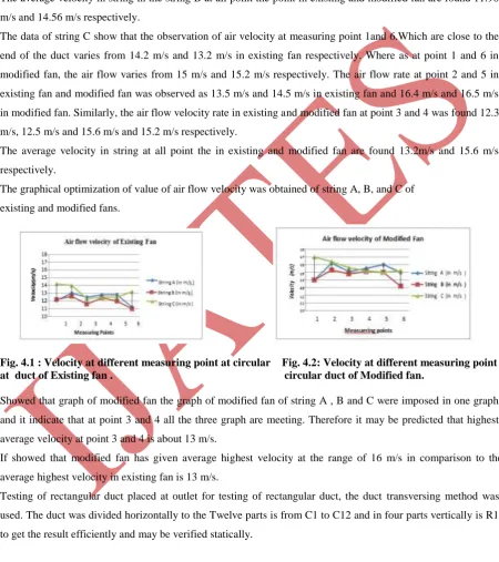
The data show that in string A, the observation of air velocity at point 1 and 6 which are closed to the end of the

duct varies from 12.1 m/s and 11.2 m/s in existing fan respectively, where as the point 1and 6 in modified fan,

the air flow velocity varies from 14 m/s and 15 m/s respectively. The velocity at the point 2 and 5 in the existing

fan was observed 13 m/s and 12 m/s respectively where as in the modified fan, the air flow velocity at point 3

and 4 points the modified fan where as the air velocity in 2 and 4 points in modified fan was observed at the rate

of 15.1 m/s and 15.5 m/s respectively, the average air flow velocity in the string A was observed in the existing

fan the rate of 12.4 m/s where as the average air flow velocity in the modified fan was observed at the rate of

15.26 m/s which is desired one.

The string is also divided in six parts take the data statically to represent all the point of the duct and compared

the air flow velocity of the duct of the existing fan and modified fan. The data were taken 1, 2,3,4,5 and 6

283 |

P a g e

the point 1 and 6 is the modified fan was observed 14 m/s and 13.2 m/s respectively.

The air flow rate at the point 2 and 5 in existing fan and modified fan was recorded as 13.6 m/s and 12 m/s in

existing fan and 15.3 m/s and 15 m/s in modified fan. Similarly the air flow velocity rate in existing and

modified fan at point 3 and 4 was found 11.6 m/s, 12.4 m/s and 14.8, 15.1 m/s respectively.

The average velocity in string in the string B at all point the point in existing and modified fan are found 11.96

m/s and 14.56 m/s respectively.

The data of string C show that the observation of air velocity at measuring point 1and 6.Which are close to the

end of the duct varies from 14.2 m/s and 13.2 m/s in existing fan respectively. Where as at point 1 and 6 in

modified fan, the air flow varies from 15 m/s and 15.2 m/s respectively. The air flow rate at point 2 and 5 in

existing fan and modified fan was observed as 13.5 m/s and 14.5 m/s in existing fan and 16.4 m/s and 16.5 m/s

in modified fan. Similarly, the air flow velocity rate in existing and modified fan at point 3 and 4 was found 12.3

m/s, 12.5 m/s and 15.6 m/s and 15.2 m/s respectively.

The average velocity in string at all point the in existing and modified fan are found 13.2m/s and 15.6 m/s

respectively.

The graphical optimization of value of air flow velocity was obtained of string A, B, and C of

existing and modified fans.

Fig. 4.1 : Velocity at different measuring point at circular Fig. 4.2: Velocity at different measuring point at duct of Existing fan . circular duct of Modified fan.

Showed that graph of modified fan the graph of modified fan of string A , B and C were imposed in one graph

and it indicate that at point 3 and 4 all the three graph are meeting. Therefore it may be predicted that highest

average velocity at point 3 and 4 is about 13 m/s.

If showed that modified fan has given average highest velocity at the range of 16 m/s in comparison to the

average highest velocity in existing fan is 13 m/s.

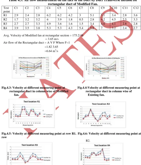
Testing of rectangular duct placed at outlet for testing of rectangular duct, the duct transversing method was

used. The duct was divided horizontally to the Twelve parts is from C1 to C12 and in four parts vertically is R1

to get the result efficiently and may be verified statically.

Table 4.2: Air flow measurement on the face of the Duct by Duct Transverse method for

rectangular duct of Existing Fan.

Test point

284 |

P a g e

R1 2.2 2 2.1 5 5.1 3 2.5 4.5 4.2 2.8 2.2 3.1

R2 1.4 2.5 2.8 5.5 3 1.5 0.4 1.3 2.9 2.8 1.5 2.5

R3 2.3 2.2 2.3 3.5 2.6 1 1.5 2.7 3.5 3.2 2.2 2.3

R4 3.1 3 2.9 2.5 5 4 4.3 4.7 6.5 2.1 1.8 2

Avg. Velocity of Exiting fan at rectangular section = 140/48 = 2.91 m/s

Air flow of the Rectangular duct = A V F Where F=1 =1.82 2.91 =5.3 m3/s

Table 4.3: Air flow measurement on the face of the Duct by Duct Transverse method for

rectangular duct of Modified Fan.

Test point

C1 C2 C3 C4 C5 C6 C7 C8 C9 C10 C11 C12

R1 2.9 2.4 2.8 6.2 6.2 4.2 3 5.1 5.1 3.4 2.8 3.6

R2 1.7 3.2 3.2 6 3.9 1.8 0.5 2.8 4.2 4.5 2.5 3.3

R3 2.7 2.7 3.3 4.9 3.6 1.6 1.5 3.4 4.6 4.1 2.8 2.8

R4 3.9 3.5 3.8 5.3 5.3 4.3 5.4 5.8 7 3.2 2.4 2.7

Avg. Velocity of Modified fan at rectangular section = 175.2/48 = 3.65 m/s

Air flow of the Rectangular duct = A V F Where F=1 =1.82 3.65

=6.64 m3/s

Fig.4.3: Velocity at different measuring point at Fig.4.4:Velocity at different measuring point at rectangular duct in column wise of Modified rectangular duct in column wise of fan. Existing fan.

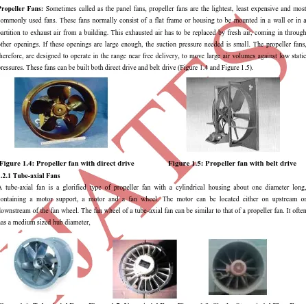
Fig.4.5: Velocity at different measuring point at row R1. Fig.4.6: Velocity at different measuring point at row

R2.

285 |

P a g e

Fig.4.9: Velocity at different measuring point at Fig.4.10: Velocity at different measuring point at rectangular duct in row wise of Modified fan rectangular duct in row wise of Existing fan.

Test was conducted to take observation on rectangular duct of modified. The data from C1 to C12 at R1 varied

from 2.4 m/s to 6.2 m/s and 1.7 m/s to 6 m/s. The value of air flow velocity from C1 to C12 at R3 and R4 varied

from 1.5 m/s to 4.9 m/s where as at R4 varied from 2.4 m/s to 7 m/s. It show that maximum value of air flow

velocity obtained at C4 and C5 with corresponding to R1 and R4.

Similarly the test was conducted to take observation rectangular duct of modified fan. The data showed that

from C1 to C12 at R1 point, the air flow velocity varied from 2 m/s to 5.1 m/s . Where 1 m/s to 3.2 m/s and 2

m/s to 5 m/s respectively.

The maximum value of air flow velocity at existing fan was obtained at C4 and C5 at corresponding to R1 is 5

to 5.1 m/s.

The data show that the maximum air flow velocity is obtained in the middle of the rectangular duct in Existing

fan as well as modified fan.

V CONCLUSION & FUTURE SCOPE

The data of air flow velocity in terms of bar diagram is presented in fig. 5.3m .The result showed that the

maximum volume of air flow rate is obtained in existing, required and modified fan are 5.994 m3/ s, 7 m3/s and

7.65 m3/ s respectively. The testing result showed that the cooling effect was obtained maximum with modified

fan air flow volume 7 m3/s.

Series 1

286 |

P a g e

Fig .5.1: A bar chart of Air flow volume of Existing fan, required fan and modified fan.

5.1 Future Scope

In the present distribution work, the detailed design procedure for an axial flow fan of heat exchanger

application has been presented experimental studies have also been performed for evaluating the performance of

the axial flow fan and necessary modification for required air flow velocity is also carried out. The testing of the

modified axial flow fan was done and desired air flow rate was obtained.

In future some mathematical model may be developed for carrying out the performance evaluation of the axial

flow fan and the result may be validated form the present experimental results. The optimization of axial air

flow fan parameter may be done for the industrial use.

REFERENCES

[1]AlirezaFalahat[ISSN: 2045-7057], “Numerical and Experimental Optimization of Flow

Coefficient in Tubeaxial Fan”, International Journal of Multidisciplinary science & Engineering , Vol. 2, No. 5,

Aug. 2011.

[2]. Oday I. Abdullah, Josef Schlattmann, “Stress Analysis of Axial Flow Fan”, Adv. Theory. Appl. Mech., Vol.

5, 2012, no. 6, 263 – 275.

[3]MahajanVandana N.,* Shekhawat Sanjay P. “Analysis of Blade of axial flow fan using Ansys”, International

Journal of Advanced Engineering Technology E-ISSN 0976-3945.2012.