Statistical Methods For Truncated Survival Data

University of Pennsylvania

ScholarlyCommons

Publicly Accessible Penn Dissertations

2018

Statistical Methods For Truncated Survival Data

Lior Rennert

University of Pennsylvania, [email protected]

Follow this and additional works at:

https://repository.upenn.edu/edissertations

Part of the

Biostatistics Commons

This paper is posted at ScholarlyCommons.https://repository.upenn.edu/edissertations/2729 For more information, please [email protected].

Recommended Citation

Rennert, Lior, "Statistical Methods For Truncated Survival Data" (2018).Publicly Accessible Penn Dissertations. 2729.

Statistical Methods For Truncated Survival Data

Abstract

{Truncation is a well-known phenomenon that may be present in observational studies of time-to-event data.

For example, autopsy-confirmed survival studies of neurodegenerative diseases are subject to selection bias

due to the simultaneous presence of left and right truncation, also known as double truncation. While many

methods exist to adjust for either left or right truncation, there are very few methods that adjust for double

truncation. When time-to-event data is doubly truncated, the regression coefficient estimators from the

standard Cox regression model will be biased. In this dissertation, we develop two novel methods to adjust for

double truncation when fitting the Cox regression model. The first method uses a weighted estimating

equation approach. This method assumes the survival and truncation times are independent. The second

method relaxes this independence assumption to an assumption of conditional independence between the

survival and truncation times. As opposed to methods that ignore truncation, we show that both proposed

methods result in consistent and asymptotically normal regression coefficient estimators and have little bias in

small samples. We use these proposed methods to assess the effect of cognitive reserve on survival in

individuals with autopsy-confirmed Alzheimer’s disease. We also conduct an extensive simulation study to

compare survival distribution function estimators in the presence of double truncation and conduct a case

study to compare the survival times of individuals with autopsy-confirmed Alzheimer’s disease and

frontotemporal lobar degeneration. Furthermore, we introduce an R-package for the above methods to adjust

for double truncation when fitting the Cox model and estimating the survival distribution function.

Degree Type

Dissertation

Degree Name

Doctor of Philosophy (PhD)

Graduate Group

Epidemiology & Biostatistics

First Advisor

Sharon X. Xie

Subject Categories

STATISTICAL METHODS FOR TRUNCATED SURVIVAL DATA

Lior Rennert

A DISSERTATION

in

Epidemiology and Biostatistics

Presented to the Faculties of the University of Pennsylvania

in

Partial Fulfillment of the Requirements for the

Degree of Doctor of Philosophy

2018

Supervisor of Dissertation

Sharon X. Xie, Professor of Biostatistics

Graduate Group Chairperson

Nandita Mitra, Professor of Biostatistics

Dissertation Committee

Warren B. Bilker, Professor of Biostatistics

Kevin G. Lynch, Associate Professor of Psychiatry

STATISTICAL METHODS FOR TRUNCATED SURVIVAL DATA

c

COPYRIGHT

2018

Lior Rennert

This work is licensed under the

Creative Commons Attribution

NonCommercial-ShareAlike 3.0

License

To view a copy of this license, visit

ACKNOWLEDGEMENT

I would like to thank my dissertation advisor, Dr. Sharon X. Xie, for all of her support and

encour-agement during my time as a PhD student. I would also like to thank my committee member and

former supervisor Dr. Kevin G. Lynch for his mentorship over the years. The professors, students,

and staff in the Biostatistics Department here at Penn have provided an amazing environment to

be in, and I am very grateful for my experience here. Finally, I would like to thank my family. Among

many things, I would not be here if it were not for the love and motivation instilled in me from my

mother. My father and brothers have also provided me with great love and encouragement and

have believed in me throughout the years. Finally, I would like to thank all of my friends. While I

probably would have graduated much sooner if it weren’t for you, I would not trade the experiences

ABSTRACT

STATISTICAL METHODS FOR TRUNCATED SURVIVAL DATA

Lior Rennert

Sharon X. Xie

Truncation is a well-known phenomenon that may be present in observational studies of

time-to-event data. For example, autopsy-confirmed survival studies of neurodegenerative diseases are

subject to selection bias due to the simultaneous presence of left and right truncation, also known

as double truncation. While many methods exist to adjust for either left or right truncation, there are

very few methods that adjust for double truncation. When time-to-event data is doubly truncated,

the regression coefficient estimators from the standard Cox regression model will be biased. In

this dissertation, we develop two novel methods to adjust for double truncation when fitting the

Cox regression model. The first method uses a weighted estimating equation approach. This

method assumes the survival and truncation times are independent. The second method relaxes

this independence assumption to an assumption of conditional independence between the survival

and truncation times. As opposed to methods that ignore truncation, we show that both proposed

methods result in consistent and asymptotically normal regression coefficient estimators and have

little bias in small samples. We use these proposed methods to assess the effect of cognitive

reserve on survival in individuals with autopsy-confirmed Alzheimers disease. We also conduct

an extensive simulation study to compare survival distribution function estimators in the presence

of double truncation and conduct a case study to compare the survival times of individuals with

autopsy-confirmed Alzheimers disease and frontotemporal lobar degeneration. Furthermore, we

introduce an R-package for the above methods to adjust for double truncation when fitting the Cox

TABLE OF CONTENTS

ACKNOWLEDGEMENT . . . iii

ABSTRACT . . . iv

LIST OF TABLES . . . vii

LIST OF ILLUSTRATIONS . . . viii

CHAPTER 1 : INTRODUCTION . . . 1

CHAPTER 2 : COX REGRESSION MODEL WITH DOUBLY TRUNCATED DATA . . . 3

2.1 Introduction . . . 3

2.2 Proposed Parametric and Nonparametric Weighted Estimators . . . 6

2.3 Asymptotic Properties of Proposed Estimators . . . 11

2.4 Simulations . . . 18

2.5 Application to Alzheimer’s Disease Study . . . 22

2.6 Discussion . . . 26

CHAPTER 3 : COX REGRESSION MODEL UNDER DEPENDENT TRUNCATION . . . 29

3.1 Introduction . . . 29

3.2 Methods . . . 32

3.3 Simulations . . . 39

3.4 Application to Alzheimer’s Disease . . . 42

3.5 Discussion . . . 45

CHAPTER 4 : BIAS IN THE SURVIVAL DISTRIBUTION FUNCTION ESTIMATOR UNDER DOUBLE TRUNCATION: ACASE STUDY OF NEURODEGENERATIVE DISEASES . . . 51

4.1 Introduction . . . 51

4.2 Existing methods to adjust for double truncation . . . 54

4.4 Example: Autopsy-confirmed Alzheimer’s disease and frontotemporal lobar

degen-eration . . . 62

4.5 Discussion and Recommendations . . . 67

CHAPTER 5 : A PACKAGE FOR ANALYZINGTRUNCATEDDATA INR . . . 70

5.1 Introduction . . . 70

5.2 Statistical methodology . . . 71

5.3 Overview of the package SurvTruncation . . . 73

5.4 Conclusions . . . 81

CHAPTER 6 : DISCUSSION. . . 83

APPENDICES . . . 87

LIST OF TABLES

TABLE 2.1 : Simulation results . . . 20

TABLE 2.2 : Simulation results under misspecification of the truncation distribution . . . 21

TABLE 2.3 : Simulation results under dependent truncation structureV =U+d0. . . 22

TABLE 2.4 : Comparing low education (<16 years) and high education (≥16 years) groups 23 TABLE 2.5 : Application: Education on survival in AD . . . 24

TABLE 3.1 : Simulation results . . . 41

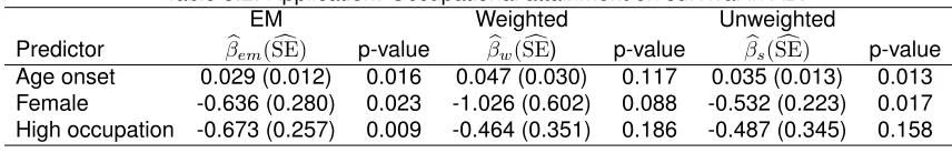
TABLE 3.2 : Application: Occupational attainment on survival in AD. . . 45

TABLE 4.1 : Simulation results . . . 59

TABLE 4.2 : Simulation results under misspecification of the truncation distribution . . . 62

TABLE 4.3 : Simulation results under violation of the independence assumption . . . 64

TABLE 4.4 : Testing equality of survival probabilities between AD and FTLD . . . 67

TABLE 5.1 : Summary of the arguments of the functioncdfDT. . . 75

LIST OF ILLUSTRATIONS

FIGURE 2.1 : Hypothetical example of double truncation . . . 4

FIGURE 2.2 : Normal Q-Q plot ofT = βbwnp−β0

b

σ from 1000 simulations under the

trunca-tion scenario for the second model described in Table 2.1 . . . 18 FIGURE 2.3 : Comparing bias and MSE (mean-squared error) of estimators . . . 21

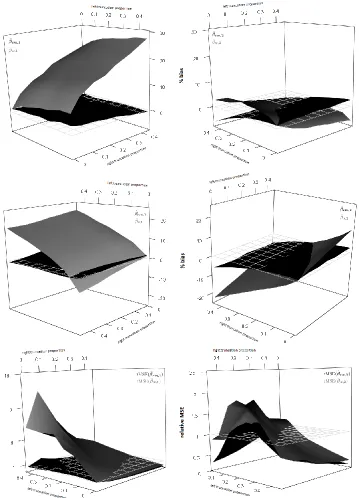
FIGURE 3.1 : Comparing bias and MSE (mean-squared error) of estimators across dif-ferent left and right truncation proportions, underdependent survival and truncation times. . . 48 FIGURE 3.2 : Comparing bias and MSE (mean-squared error) of estimators across

dif-ferent left and right truncation proportions, underindependentsurvival and truncation times. . . 49 FIGURE 3.3 : Comparing bias and MSE (mean-squared error) of estimators under

de-pendent left truncation. . . 50

FIGURE 4.1 : Schematic depiction of doubly truncated neurodegenerative disease data . 52 FIGURE 4.2 : Bias of distribution function estimators. . . 58 FIGURE 4.3 : Bias of distribution function estimators under misspecification of truncation

distribution. . . 60 FIGURE 4.4 : Bias of distribution function estimators under violation of independence

as-sumption . . . 63 FIGURE 4.5 : Estimated distribution functions for AD and FTLD . . . 66

FIGURE 5.1 : NPMLE of the cumulative distribution function and survival function of the AIDS induction times. . . 78 FIGURE 5.2 : NPMLE of the marginal cumulative distribution function of left truncation

time (left) and right truncation time (right). . . 79 FIGURE 5.3 : NPMLE of the joint cumulative distribution function of left and right

CHAPTER 1

I

Truncation is a statistical phenomenon that has been shown to occur in a wide range of applications,

including survival analysis, epidemiology, economics, and astronomy. Individuals who are subject

to truncation provide no information to the investigator. Left truncation occurs when data is only

recorded for individuals whose survival time exceeds a random time (i.e. left truncation time).Right

truncationoccurs when data is only recorded for individuals whose survival time proceeds a random

time (i.e. right truncation time). When both left and right truncation are present, this is known as

double truncation.

Double truncation is inherent in retrospective autopsy-confirmed studies of neurodegenerative

dis-eases. Due to the inaccuracy of clinical diagnosis (Beach et al., 2012), autopsy confirmation is

needed for a definitive diagnosis (Grossman and Irwin, 2016) of a particular neurodegenerative

disease. The right truncation occurs because information is only obtained from a subject when they

receive an autopsy. Subjects who survive past the end of the study are not diagnosed and therefore

not included in the study sample, resulting in a sample that is biased towards subjects with smaller

survival times. Furthermore, the retrospective sample is also left truncated because subjects who

succumb to the disease before they enter the study are unobserved, resulting in a sample that is

biased towards subjects with larger survival times. We note that right censoring is not possible in

this setting, since any subject who has an autopsy performed will also have a known survival time.

A diagram showing how double truncation occurs is provided in Figure 2.1.

The aim of our data analysis is to get accurate estimates of the effect of risk factors on survival

from disease symptom onset in subjects with autopsy-confirmed neurodegenerative diseases. The

default application for analysis in this setting is the Cox regression model (Cox, 1972). However,

regression techniques which do account for truncation will result in biased regression coefficient

estimators. This is because under left truncation, individuals with smaller event times are less

likely to be observed, resulting in a study sample that is biased towards larger event times and

risk factors associated with larger event times. Similarly, under right truncation, individuals with

smaller event times and risk factors associated with smaller event times. If double truncation is

not accounted for, then the regression coefficient estimators from the Cox regression model will be

biased.

In Chapter 2, we introduce a weighted estimating equation approach to adjust the Cox regression

model in the presence of double truncation, under the assumption that the survival times and

trun-cation times are independent. In chapter 3, we use a conditional likelihood approach to relax this

independence assumption to an assumption of conditional independence between the survival and

truncation times. Here we estimate the regression coefficient estimators for the Cox regression

model using an expectation-maximization (E-M) algorithm. In Chapter 4, we conduct a case study

to compare estimators of the survival distribution function under double truncation. In Chapter 5, we

introduce an R-package to adjust both the Cox regression model and the survival time distribution

function in the presence of double truncation. The R-package is intended for the situation where

the survival and truncation times are independent. Concluding remarks are given in Chapter 6. The

code for the Cox regression coefficient estimators using the EM algorithm introduced in Chapter 3 is

provided in Appendix D. The code for the functions contained in the R package described in

Chap-ter 5, which use a nonparametric weighting approach to adjust the Cox regression model (ChapChap-ter

CHAPTER 2

C

2.1. Introduction

Accurate regression coefficient estimation in survival analysis is crucial for studying factors that

affect disease progression. However in some survival studies the outcome of interest may be

subject to either left or right truncation. When both left and right truncation are present, this is known

as double truncation. For example, double truncation is inherent in retrospective autopsy-confirmed

studies of Alzheimer’s disease (AD), where autopsy confirmation is the gold standard for diagnosing

AD due to the inaccuracy of clinical diagnosis (Beach et al., 2012). The right truncation occurs

because information is only obtained from a subject when they receive an autopsy. Subjects who

survive past the end of the study are not diagnosed and therefore not included in the study sample,

resulting in a sample that is biased towards subjects with smaller survival times. Furthermore, the

retrospective sample is also left truncated because subjects who succumb to the disease before

they enter the study are unobserved, resulting in a sample that is biased towards subjects with

larger survival times. We note that right censoring is not possible in this setting, since any subject

who has an autopsy performed will also have a known survival time.

A diagram showing how double truncation occurs is provided in Figure 2.1. In this hypothetical

example, we assume subjects 1, 2, and 3 all have similar times of disease symptom onset. For

illustrative purposes, we also assume that subjects 1, 2, and 3 have the same study entry time,

however this need not be the case. Here the x-axis represents time, and the squares represent the

terminating events. Subject 1 is left truncated because they die before they enter the study. Subject

2 enters the study and dies before the end of the study, and is therefore observed. Subject 3 is

right truncated because they live past the end of the study, and therefore do not have an autopsy

performed.

If the left and right truncation are not accounted for then the observed sample will be biased,

which may lead to biased estimators of regression coefficients and hazard ratios. In this paper, we

examine the relationship between education and survival from AD symptom onset in a retrospective

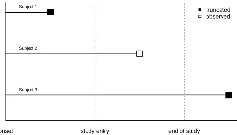
Figure 2.1: Hypothetical example of double truncation

onset study entry end of study

Subject 1

Subject 2

Subject 3

truncated observed

In this hypothetical example, we assume subjects 1, 2, and 3 all have similar times of disease symptom onset. For illustrative purposes, we also assume that subjects 1, 2, and 3 have the same study entry time, however this need not be the case. Here the x-axis represents time, and the squares represent the terminating events. Subject 1 is left truncated because they die before they enter the study. Subject 2 enters the study and dies before the end of the study, and is therefore observed. Subject 3 is right truncated because they live past the end of the study, and therefore do not have an autopsy performed.

regression model (Cox, 1972). However, to obtain consistent regression coefficient estimators,

we must adjust for truncation. Regression techniques already exist under left truncation (Lai and

Ying, 1991), right truncation (Kalbfleisch and Lawless, 1991), and length-biased data (Wang, 1996).

In this paper, we propose a Cox regression model to adjust for double truncation using a weighted

estimating equation approach, where the hazard rate for the failure times follows that of the standard

Cox regression model.

Although double truncation may appear in many studies in which data is only recorded for subjects

whose event times fall in an observable time interval, the amount of literature on methods to handle

double truncation is small. Most of the literature deals with the estimation of the survival distribution

rather than regression. Efron and Petrosian (1999) introduced the nonparametric maximum

likeli-hood estimator (NPMLE) for the survival distribution function under double truncation. Shen (2010)

investigated the asymptotic properties of the NPMLE and introduced a nonparametric estimator of

the truncation distribution function. Shen (2010) and Moreira and de ˜Una- ´Alvarez (2010) introduced

a semiparametric maximum likelihood estimator (SPMLE) for the survival distribution function under

and doubly truncated data using linear transformation models, but these models only allow discrete

covariates and the asymptotic properties of the resulting estimators are not established. Moreira,

de ˜Una- ´Alvarez, and Meira-Machado (2016) introduced nonparametric kernel regression for doubly

truncated data, where a mean function conditional on a single covariate is estimated, rather than a

hazard ratio. Furthermore, the resulting estimator is asymptotically biased. Since right censoring is

rare under double truncation, the current literature assumes no censoring or interval censoring.

The concept of adjusting the Cox regression model for biased samples using a weighted estimating

equation approach was first introduced by Binder (1992) for survey data. In this setting, the weights

were knowna priori and a biased study sample was selected directly from the target population

(i.e. the population we wish to study). Lin (2000) proved the asymptotic normality of the regression

coefficient estimator introduced by Binder, and extended the model to settings where the biased

study sample is selected from a representative sample of the underlying target population. Pan

and Schaubel (2008) introduced a Cox regression model with estimated weights, using logistic

regression to estimate each subject’s probability of selection into the study. In their setting, they

assumed that baseline information was available from both subjects with observed and missing

survival times. Due to truncation, we do not have any information on subjects with missing survival

times. Therefore previous methods are unable to address the unique challenges present in our AD

study.

There are several new contributions of this paper to the literature. We propose a Cox regression

model using a weighted estimating equation approach to obtain a hazard ratio estimator under

dou-ble truncation, where the weights are inversely proportional to the probability that a subject isnot

truncated. These selection probabilities are estimated both parametrically and nonparametrically

using methods introduced by Shen (2010a, 2010b) and Moreira and de ˜Una- ´Alvarez (2010). As

opposed to using data from missing subjects, the selection probabilities here are estimated using

survival and truncation times from observed subjects only. The parametric selection probabilities

make distributional assumptions about the truncation times, while the nonparametric selection

prob-abilities do not. We show that the proposed regression coefficient estimators are consistent, and

greatly reduce the bias in finite samples compared to the standard Cox regression estimator which

ignores double truncation. We prove the asymptotic normality of the regression coefficient

use the bootstrap technique (Efron and Tibshirani, 1993) to estimate the variance and confidence

intervals of the regression coefficient estimator under nonparametric weights.

The remainder of this paper is organized as follows. In Section 2.2 we introduce the weighted

esti-mating equation and the proposed estimators, as well as the estimation procedure for the weights.

The asymptotic properties of the proposed estimators are provided in Section 2.3. In Section 2.4

we conduct a simulation study to assess the finite sample performance of the proposed estimators.

The proposed method is then applied to the AD data in Section 2.5. Discussion and concluding

remarks are given in Section 2.6.

2.2. Proposed Parametric and Nonparametric Weighted Estimators

Throughout this paper, we refer topopulation random variablesas random variables from the target

population and denote them without subscripts. We refer tosampling random variablesas random

variables from the observed sample and denote them with subscripts. These two sets of variables

may have different distributions due to double truncation, which is why standard methodology may

be inappropriate.

LetTi denote the observed survival times for subjecti = 1, ..., n ≤N, wherenis the size of the

observed sample andN is the size of thetarget sample. Here we use the term target sample to

denote a representative sample from the underlying target population. In our setting, this consists

of all subjects that would have been included in the observed sample had truncation not occurred.

For a given timet, defineYi(t) = 1{Ti≥t}andNi(t) = 1{Ti≤t}. Letτ be a constant set to the end of

study time. The Cox regression model assumes that for a given subject withp×1covariate vector

Zi(t), the hazard function at timetis given byλi(t) =λ0(t)eβ

0

0Zi(t)_{, whereλ}

0(t)is the true baseline

hazard function and is unspecified. The truep×1regression coefficient vector,β₀, is estimated by

b

β, the solution to

U(β) = n

X

i=1

Z τ

0

Zi(t)−

Pn

j=1Yj(t)eβ

0_Z j(t)_Z

j(t)

Pn

j=1Yj(t)eβ

0_Z j(t)

dNi(t) =0, (2.1)

wheredNi(t) =Ni(t)−Ni(t−). Since right censoring is not possible under our sampling scheme,

we do not include it in the estimation procedures. Therefore dNi(Ti)= 1 in this setting, since all

When subjects have unequal probabilities of selection, then the study sample will not be a

repre-sentative sample of the underlying target population. To adjust for biased samples, Binder (1992)

proposed weighting each subject in the score equation 2.1 by the inverse probability of their

inclu-sion in the sample. The true regresinclu-sion coefficientβ₀is then estimated byβb_w, the solution to the

weighted score equation

Uw(β,π) =

n

X

i=1

Z τ

0

wi

Zi(t)−

Pn

j=1wjYj(t)eβ

0_Z j(t)_Z

j(t)

Pn

j=1wjYj(t)eβ

0_Z j(t)

dNi(t) =0. (2.2)

Here π = (π1, ..., πn) and wi = π−i 1, where πi is the selection probability for subject i, and is

conditional on subject specific characteristics. The method described above assumes that the

selection probabilitiesπiare knowna priori. When these probabilities are not known, they must be

estimated.

In our setting, we can estimate the probability that a subject was selected in our sample (i.e. not

truncated), conditional on their observed survival time. Thus a natural solution to adjust for double

truncation is to use these estimated selection probabilities in (2). These selection probabilities are

estimated using the survival and truncation times from observed subjects only. The estimation

procedure is given in Section 2.2.1.

In our data example, the left truncation time is taken to be the time from AD symptom onset to

entry into the study. The right truncation time is set to the time from AD symptom onset to the end

of the study. LetU and V denote the left and right truncation times, respectively. Due to double

truncation, we observe{T, U, V,Z(t)}if and only ifU ≤T ≤V.

Conditional onTi, subjecti is observed with probabilityπi =P(U ≤ T ≤ V|T =Ti). Hereπi is

the probability that a subject from the target sample with survival timeT =Ti is observed, and is

called the selection bias function (Bilker and Wang, 1996). For an intuition as to why this weighting

scheme works, we consider the following. Ifxindividuals with survival timeTiare observed in the

sample, then by the definition ofπi, there must bex/πiindividuals in the target sample with survival

timeTi. Without loss of generality, supposex= 1, so that there are 1/πi individuals with survival

time Ti in the target sample. Of these, (1/πi)×πi = 1will be observed and the other 1/πi −1

individuals are referred to as ghosts (Turnbull, 1976) and are unobserved. In this case, eachTi

adjust for the biased sample by weighting each observation in the estimating equation 2.1 by1/πi.

To give another intuitive view as to how the weighting works, it can be shown thatπiis proportional

to the probability of observing a survival timeTiin the observed sample relative to the probability of

observing a survival timeTiin the target sample. That is,πi∝P(T =Ti|U ≤T ≤V)/P(T =Ti).

Using these selection probabilities in (2) works because observations with survival times which are

oversampled in the observed sample relative to the target sample are downweighted and those

which are undersampled are upweighted, yielding a score function consisting of survival times (and

corresponding covariates) that are distributed according to those of the target population. We show

in Section 2.3 that if these selection probabilities are estimated consistently and plugged into the

score equation 2.2, then this score function is asymptotically equivalent to the unweighted score

function using all observations from the target sample, and is therefore asymptotically unbiased.

This results in the consistency of the proposed regression coefficient estimators presented below.

2.2.1. Estimation of selection probabilities

The methods used to estimate the selection probabilities assume that the survival and truncation

times are independent in the observable region U ≤ T ≤ V. This independence assumption is

needed to estimateπ using the estimation procedures below. We note that under independence,

πi is simplyP(U ≤ Ti ≤ V). Situations where the independence assumption can be relaxed by

covariate adjustment are discussed in Section 2.6.

Before we describe the parametric and nonparametric procedures for estimating the selection

prob-abilities, we introduce additional notation and assumptions. Letf(t)andF(t)denote the density

and cumulative distribution functions of T. Let k(u, v) and K(u, v) denote the joint density and

cumulative distribution functions of (U, V). For any cumulative distribution function H, define the

left endpoint of its support by aH = inf{x : H(x) > 0} and the right endpoint of its support by

bH = inf{x : H(x) = 1}. Let HU(u) = K(u,∞) and HV(v) = K(∞, v) denote the marginal

cumulative distribution functions ofU andV, respectively. For the following methods, we assume

thataHU < aF ≤aHV andbHU ≤bF < bHV. These conditions are needed for identifiability of the

selection probability estimators presented below (Shen, 2010a,b; Woodroofe, 1985).

Lettingπ(t) =P(U ≤t≤V), our methods rest on the assumption thatπ(t)>0for allt∈[aF, bF].

of this positivity assumption can lead to aπi that is very small and thus gives undue influence to

theith_{observation in the score equation 2.2. We discuss a remedy to this situation at the end of}

Section 2.6. We note that this positivity assumption is generally implied through the identifiability

constraintsaHU < aF ≤aHV andbHU ≤bF < bHV. Justification of these constraints and positivity

assumption for our data example, and a discussion on when these may be violated, are given in

Web Appendix D.

Nonparametric estimation

We now present the nonparametric estimation of the selection probabilitiesπi. As shown in Shen

(2010a, p. 837), the distribution of the observed survival times, F˜(t), can be written as F˜(t) =

P(Ti≤t) =P(T ≤t|U ≤T ≤V) =p−1P(T ≤t, U ≤T ≤V) =p−1

Rt

0[K(s, bHV)−K(s, s)]F(ds),

wherep=P(U ≤T ≤V)is the probability of observing a random subject from the target sample.

The last equality follows from the independence ofT and(U, V)in the observable regionU ≤T ≤

V. In this case, the density of the observed survival times is given byf˜(t) =p−1_{×π(t)f(t), where}

π(t) = K(t, bHV)−K(t, t) = P(U ≤t ≤V). It can also be shown that under this independence

assumption, the joint density of the observed truncation times can be written ask˜(u, v) = p−1_×

ϕ(u, v)k(u, v), whereϕ(u, v) =F(v)−F(u−) =P(u≤T ≤v).

Letϕ= (ϕ1, ..., ϕn), whereϕi =ϕ(Ui, Vi). Sincek(u, v) =p×k˜(u, v)/ϕ(u, v), we have that when

ϕ andpare known, K(u, v) can be estimated byn−1_pPn

j=1

1{Uj≤u,Vj≤v}

ϕj . Settinguand v to ∞,

we can estimate p by n Pn j=11/ϕj

−1

. Therefore when ϕ is known, we can estimate K(u, v)

by Pn j=11/ϕj

−1Pn

j=1

1{Uj≤u,Vj≤v}

ϕj and thus πi = K(Ti, bHV)−K(Ti, Ti) can be estimated by

Pn j=11/ϕj

−1Pn

j=1

1{_Uj≤_Ti≤_Vj}

ϕj . Similarly, sincef(t) = p× ˜

f(t)/π(t), we have that when π is

known,F(t)can be estimated by Pn j=11/πj

−1Pn

j=1 1{_Tj≤t}

πj and thusϕi=F(Vi)−F(Ui−)can

be estimated by Pn j=11/πj

−1Pn

j=1

1{_Ui≤_Tj≤_Vi}

πj .

Shen (2010) proved that the NPMLE’s of ϕi andπi, denoted byϕ_bi andπ_bi, respectively, can be

found using the following iterative algorithm:

Step 0) Setϕ_b(0)_i =n−1Pn

j=11{Ui≤Tj≤Vi}, fori= 1, ..., n.

Step 1) Set_bπ_i(1)=Pn

j=1 1

b

ϕ(0)_j

−1 Pn

j=1

1{Uj≤Ti≤Vj}

b

Step 2) Setϕ_b(1)_i =Pn

j=1 1

b

π(1)_j

−1 Pn

j=1

1{_Ui≤_Tj≤_Vi}

b

π_j(1) , fori= 1, ..., n.

Step 3) For a prespecified errore, repeat steps 1 and 2 untilPn

i=1|bπ

(s) i −πb

(s−1) i |< e.

The NPMLE of π is given by π_bnp = (_bπ₁(s), ...,π_b(s)n ), with estimated weights wnp = 1/πb

np

. The

corresponding estimator ofβ₀is denoted byβb_w

np, the solution toUw(β,πb

np ) =0.

Because we do not need estimates of the survival and truncation time distributions, the algorithm

to estimateπpresented here is a simplified version of the algorithm given in Shen (2010). We note

that both algorithms result in the same estimatorπ_bnp.

Parametric estimation

We can also estimate the selection probabilities parametrically using the methods introduced by

Shen (2010) and Moreira and de ˜Una- ´Alvarez (2010). In this setting, we assume that the truncation

timesU andV have a parametric joint density functionkθ(u, v). Here θ ∈ Θ is aq×1vector of

parameters andΘis the parametric space.

Under the assumption of independence in the region U ≤ T ≤ V, the conditional likelihood of

the(Ui, Vi)given Ti is given byLc(θ) = Qn_i=1kθ(Ui, Vi)/πiθ, whereπθi =

R

u≤Ti≤vkθ(u, v)dudv =

Pθ(U ≤Ti≤V). Here the subscriptθdenotes that the probability depends onθ. In this setting, we

estimateπi byπbθi =

R

u≤Ti≤vkθb(u, v)dudv. The conditional likelihood estimator,θb, is the solution to

Uc(θ) = _∂∂_θlogLc(θ) =0.

The MLE ofπis given byπbθ_{= (π}bθ

1, ..., πθnb). The weightswiare then estimated bywi(bθ) =p(bθ)/πbθ_i,

wherep(bθ) =P b

θ(U ≤T ≤V) = n

−1Pn

j=11/π

b θ

j

−1

. The corresponding estimator ofβ₀is denoted

by βb_w

b

θ, the solution to Uw(β,π b

θ_{) =0. Here the estimated parametric weightsw}

i(bθ)scale1/πbθ_i

byp(bθ)so that they sum up to the original sample sizen, which is needed for the derivation of the

asymptotic variance ofβb_w

b

θ.

2.2.2. Estimating the regression coefficients

The estimated parametric and nonparametric selection probabilities,πbθ andπb

np

, can be computed

using the code provided in the online supplementary materials. The regression coefficient

estima-torsβb_w

b

R (coxph) with weights p(bθ)/πbθ and1/π_b

np

. More details, including standard error estimates and

confidence intervals ofβb_w

b

θ andβbwnp, as well as sample data, are provided in our code.

2.3. Asymptotic Properties of Proposed Estimators

In this section, we describe the asymptotic properties of our proposed estimatorsβb_wnp andβb_w

b

θ. The asymptotic properties of the proposed estimators refer to the situation when the total number

of observed (non-truncated) subjectsn → ∞. The following theorems assume that the regularity

conditions listed below hold.

The regularity conditions listed here are adapted from Andersen and Gill (1982), Pan and Schaubel

(2008), and Shen (2010ab). For ap×1vectora, we denotea⊗0_{= 1,a}⊗1_{=a, anda}⊗2_{as thep×p}

matrixaa0. Conditions (a)-(f) below are needed for the consistency ofβb_w

np:

(a){Ti, Ui, Vi,Zi}are independent and identically distributed fori= 1, ..., N,

(b)Rτ

0 dΛ0(t)<∞, whereΛ0(t)is the baseline cumulative hazard function,

(c) ForSw(j)(β,π;t) =n−1Pn_i=1π−i1Yi(t)eβ

0_Z i(t)_Z

i(t)⊗j,j= 0,1,2, we assume the existence of a

neighborhoodB0ofβ0andΠ0ofπ0such thatsupt∈[0,τ],β∈B0,π∈Π0kSw (j)

(β,π;t)−sw(j)(β,π;t)k

p

−→0asn→ ∞, forj= 0,1,2, wheresw(j)(β,π;t)=E{Sw(j)(β,π;t)}ands

(0)

w (β,π;t)>0,

(d) There exists aδ >0such thatπ(t) =P(U ≤t≤V)> δalmost surely for everyt∈[aF, bF],

(e)Rτ

0 |Zik(t)|dt <∞almost surely, whereZik(t)is thek

th_{covariate value for subjectiat timet,}

(f) The Cox model assumptionλ(t) = λ0(t)eβ

0

0Z(t)holds for both observed and unobserved

sub-jects.

Condition (a) is used when applying the central limit theorem, and this assumption is reasonable

in practice assuming the subjects are independent. Condition (b) is used to ensure that several

terms in the proofs of Theorems 2.1 and 2.2 are bounded. Condition (c) ensures thatSw(j)(β,π;t)

converges in probability, and thate(β,π;t) = sw(1)(β,π;t) s(0)w(β,π;t)

is bounded. This assumption is applied

several times throughout the proofs below. Condition (d) states that the probability of observing

any survival timetin[0, τ]is non-zero, which leads to the boundedness of several quantities in the

proofs below and ensures thatN andngo to∞at the same rate. Condition (e) is a boundedness

condition of the covariateZik(t). While it is not required, it is applicable in most situations and is

used to simplify the proofs of Theorems 2.1 and 2.2. For a fixed covariate vectorZ(t)and fixed time

Cox model) regardless of whether a subject was observed or truncated. This assumption is used

implicitly in the proof of Theorem 2.1 when concluding N−1_U

w(β,πb)andN

−1_U∗_(β)

(defined in

the proof of Theorem 2.1) converge to the same limit.

For the consistency ofβb_w

b

θ, we need the following three conditions in addition to (a)-(f): (g)Gθ(t) =Pθ(U ≤t≤V) =R

u≤t≤vkθ(u, v)dudvis continuous intfor everyθ∈Θ,

(h)θbn p −

→θimpliesG b θn(t)

p

−→Gθ(t)for everyt∈[0, τ],

(i) Existence of a neighborhoodB0ofβ0andΘ0ofθ0such thatsupt∈[0,τ],β∈B0,θ∈Θ0kSw (j)

(β,θ;t)

−sw(j)(β,θ;t)k

p

−→0asn→ ∞, forj = 0,1,2, wheresw(j)(β,θ;t)=E{Sw(j)(β,θ;t)}and

s(0)w (β,θ;t)>0. The quantitySw(j)(β,θ;t)is defined in the proof of Theorem 2.2.

Conditions (g) and (h) are used for the uniform consistency ofπbθ

i toπ

θ0

i across all possible values of

Tiin[0, τ]. Note thatπiθ=Gθ(Ti). Condition (i) ensures thatSw(j)(β,θ;t)converges in probability,

and thate(β,θ;t) = sw(1)(β,θ;t)

s(0)w (β,θ;t)

is bounded.

The regularity conditions (j) and (k) below are needed in addition to (a)-(i) for the asymptotic

nor-mality ofβb_w

b

θ:

(j) For everyt∈[0, τ]andθin a neighborhoodΘ0ofθ0,Gθ(t)is continuously differentiable inθ,

(k) Positive-definiteness of the matricesAw(β,θ)andI(θ)(defined in proof of Theorem 2.2).

Condition (j) is used to ensure the existence of Q(β0,bθ) defined in the proof of Theorem 2.2,

along with its convergence toQ(β0,θ0). Condition (k) ensures the existence of the inverses of the

matricesAw(β,θ)andI(θ).

Theorem 2.1:βb_w

npandβbwθb

are consistent estimators ofβ₀asn→ ∞.

Proof of Theorem 2.1: The following proof holds for bothw_b = wnpand w_b = w_bθ. We therefore

denoteπ_bnpandπbθ_by b

π to simplify notation in this setting. The score equation 2.2 can be written

as

Uw(β,π) =

N X i=1 Z τ 0 ξi πi

{Zi(t)−Ew(β,π;t)}dNi(t), (2.3)

whereEw(β,π;t) = PN_j=1ξ_πj

jYj(t)e

β0Zj(t)_Z

j(t) /PN_j=1ξ_πj

jYj(t)e

β0Zj(t) _{, andξ}

i is an indicator

from both truncated and observed subjects, withξi= 0 for truncated subjects.

Letβb b

wbe the solution toUw(β,πb) =0. We will show thatN

−1_U

w(β,πb)andN

−1_U∗_(β)

converge

to the same limit, where U∗(β) = PN

i=1

Rτ

0{Zi(t)−E(β;t)}dNi(t) is the complete case score

function which includes all observations from both truncated and observed subjects, andE(β;t) =

PN

j=1{Yj(t)e

β0Zj(t)_Z

j(t)}/P_j=1N {Yj(t)eβ

0_Z

j(t)_{}. We then apply results from Lin (2000) and convex}

function theory to conclude thatβb b

w p −→β₀.

Forπ(t) =P(U ≤t≤V), Shen (2010a,2010b) proved that_bπ(t)converges uniformly in probability

(with respect to t) to π0(t). Here πb(t) denotes the estimator of π(t) under both parametric and

nonparametric assumptions, andπ0(t) is the true probability of observing a subject with survival

timet. We will denoteπ_biandπ0,ias the estimated and true probability of observing a subject with

survival timeTi, respectively. Note thatπbi=bπ(Ti)andπ0,i=π0(Ti).

We can re-expressN−1_U

w(β,πb)as

N−1Uw(β,πb) =N

−1 N X i=1 Z τ 0

π_0,i−1ξi{Zi(t)−Ew(β,πb;t)}dNi(t) (2.4)

+N−1

N

X

i=1

Z τ

0

{π_b−_i1−π_0,i−1}ξi{Zi(t)−Ew(β,π_b;t)}dNi(t). (2.5)

We will now state and prove a lemma used throughout the proof of Theorem 2.1.

Lemma:N−1PN

i=1(bπ

−1

i −π

−1

0,i)g(·) p

−→0for any stochastically bounded functiong.

Proof: LetHN(πb;·) =N

−1PN

i=1(bπ

−1

i −π

−1

0,i)g(·). We need to show that∀ >0,∃N ≥Nsuch that

P(|HN(π_b;·)|> )< .

By the uniform consistency of_bπ(t)int fort ∈ [aF, bF]and the continuous mapping theorem, we

have thatπ_b−1_{(t)is also uniformly consistent int fort ∈ [a}

F, bF]. That is, ∀ > 0,∃N1 such that

N ≥N1 =⇒ P( sup t∈[aF,bF]

|π_b−1(t)−π−₀1(t)| > )< . Sincegis stochastically bounded,∃M <∞

andN2 such that∀ >0, N > N2 =⇒ P(|g(·)|> M)< .

P(|HN(πb;·)|> ) =P(N −1 | N X i=1

(π_bi−1−π_0,i−1)g(·)|> )

≤P(N−1

N

X

i=1

|(_bπ−_i1−π_0,i−1)g(·)|> )≤P(N−1

N

X

i=1

|_bπ_i−1−π_0,i−1|> /M)

≤P( max

i=1,..,N|bπ

−1

i −π

−1

0,i|> /M)≤P( sup t∈[aF,bF]

|π_b−1(t)−π₀−1(t)|> /M)< .

Forj= 0,1, we can write

Sw(j)(β,πb;t) =N

−1

N

X

i=1

π−_0,i1ξiYi(t)eβ

0_Z i(t)_Z

i(t)⊗j+N−1 N

X

i=1

(_bπ_i−1−π_0,i−1)ξiYi(t)eβ

0_Z i(t)_Z

i(t)⊗j

SinceZi(t)is stochastically bounded by regularity assumption (e), the termξiYi(t)eβ

0_Z i(t)_Z

i(t)⊗j

is also stochastically bounded. Application of the lemma therefore yieldsSw(j)(β,πb;t) =

Sw(j)(β,π0;t) +op(1). SinceEw(β,πb;t) =

Sw(1)(β,πb;t) Sw(0)_(β,

b

π;t), application of Slutsky’s theorem yields

Ew(β,πb;t) =Ew(β,π0;t) +op(1).

We therefore have that 2.4 is equivalent toN−1PN

i=1

Rτ

0 π

−1

0,iξi{Zi(t)−Ew(β,π0;t) +op(1)}dNi(t).

Equation 2.5 is equivalent toN−1PN

i=1

Rτ

0{bπ

−1

i −π

−1

0,i}ξi{Zi(t)−Ew(β,π0;t) +op(1)}dNi(t), which

converges in probability to0by the lemma.

Finally, another application of Slutsky’s theorem yields

N−1Uw(β,πb) =N

−1 N X i=1 Z τ 0

π_0,i−1ξi{Zi(t)−Ew(β,π0;t)}dNi(t) +op(1) =N−1Uw(β,π0) +op(1).

Thus N−1Uw(β,πb) and N

−1_U

w(β,π0) converge to the same limit. Since N−1Uw(β, π0) and

N−1_U∗_(β)

converge to the same limit (Lin 2000), N−1_U

w(β,πb) andN

−1_U∗_(β)

must also

con-verge to the same limit. Therefore our proposed estimating equation,Uw(β,πb), is asymptotically

equivalent to the standard Cox estimating equation containing all of the observations from the target

sample,U∗(β). SinceU∗(β)is maximized atβ₀(Andersen and Gill 1982), it follows from convex

function theory thatβb b w

p

−→β₀(Lin 2000).

Theorem 2.2Under correct specification of the truncation distribution,√n(βb_w

b

asymptoti-cally normal asn→ ∞with mean zero and covariance matrix

Σ(β₀,θ0) =Aw(β0,θ0)−1Vw(β0,θ0)Aw(β0,θ0)−1.

To estimate the asymptotic variance of βb_w

ˆ

θ, we need some additional definitions. Let wi(θ) = p(θ)/πθ

i, wherep(θ) =Pθ(U ≤T ≤V). Denoteθ0as the true value ofθ. For ap×1vectora,a⊗0

= 1,a⊗1_{=a, anda}⊗2_{denotes thep×pmatrixaa}0_{. Let}

dMi(β;t) =dNi(t)−Yi(t)eβ

0_Z i(t)_dΛ

0(t),wheredΛ0(t)is the hazard function,

Sw(j)(β,θ;t) =n−1

n

X

i=1

wi(θ)Yi(t)eβ

0_Z i(t)_Z

i(t)⊗j, j= 0,1,2,

Ew(β,θ;t) =Sw(1)(β,θ;t)/Sw(0)(β,θ;t),

Q(β,θ) =Eh Z τ

0

∂

∂θ˜wi(˜θ){Zi(t)−Ew(β,θ;t)}dMi(β;t)

i

|˜_θ=θ,

Uc(θ) = n

X

i=1

Uci(θ),whereUci(θ) =

∂

∂θlog(kθ(Ui, Vi)/π θ

i),

I(θ) =−Enn−1∂Uc(˜θ) ∂θ˜

o

|˜_θ=θ,

φi(β,θ) = Z τ

0

wi(θ){Zi(t)−Ew(β,θ;t)}dMi(β;t) +Q(β,θ)I(θ)−1Uci(θ),

Vw(β,θ) =E{φi(β,θ)

⊗2_},

Aw(β,θ) =E h

−

Z τ

0

wi(θ)

nS_w(2)(β,θ;t)

Sw(0)(β,θ;t) −Sw

(1)_(β,θ;t)⊗2

Sw(0)(β,θ;t)2

o dNi(t)

i ,

Σ(β,θ) =Aw(β,θ)−1Vw(β,θ)Aw(β,θ)−1.

The asymptotic variance of βb_wˆ

θ is given by Σ(β0,θ0) = Aw(β0,θ0)

−1_V

w(β0,θ0)Aw(β0,θ0)−1.

We can estimatedΛ0(t)by dΛb0(βb_w

ˆ

θ,bθ;t) =n

−1Pn

j=1wj(bθ)dNj(t)/S (0) w βb_w

ˆ

θ,θb;t

, anddMi(β;t)

by dMci(βb_w

ˆ

θ,bθ;t) = dNi(t)−Yi(t)e b β0_w

ˆ

θ Zi(t)

dΛb0(βb_w

ˆ

θ,bθ;t). It can be shown that the remaining matrices defined above can be consistently estimated by their empirical counterparts, where β₀

andθ0are replaced by their corresponding estimatorsβb_w

ˆ

θ andθb, respectively. It follows that the estimator of the asymptotic variance ofβb_w

ˆ

θ,Σ βbwˆθ,bθ

, is consistent forΣ(β₀,θ0). The derivatives

∂

∂θwi(θ),Uc(θ), and

∂Uc(θ)

∂θ can be computed directly (when possible) or numerically.

Proof of Theorem 2.2: The proof proceeds by multiple applications of Taylor’s theorem, results from

empirical processes, the multivariate central limit theorem, and Slutsky’s theorem. It can easily

counterparts using the strong law of large numbers and Slutsky’s theorem.

Using simple algebra, we rewrite the score function given in equation 2.2 in Section 2.2, with

para-metric weights, as

Uw(β,θb) =

n X i=1 Z τ 0 1

πbθ

i

{Zi(t)−Ew(β,θb;t)}dMci(β,bθ;t).

Taylor expansion ofUw(βb_w

ˆ

θ,bθ)aroundβ=β0yields

√

n(βb_wˆ

θ−β0) =

n−1∂Uw(β,bθ) ∂β

−1

|β=β∗

n−12_Uw(β 0,bθ),

whereβ∗ lies betweenβb_w

ˆ

θ andβ0 inR

p_{. The uniform convergence in probability of π}bθ _{to π}θ0_,

the consistency ofβb_w

ˆ

θ, and the continuous mapping theorem implies the uniform convergence of S(j)_w (βb_w

ˆ

θ,bθ;t)tos

(j)

w (β0,θ0;t)int, forj = 0,1,2. Application of the strong law of large numbers

yields

n−1∂Uw(β,bθ) ∂β |β=bβ_w

ˆ

θ

p −

→Aw(β0,θ0).

Applying the mean value theorem yields

√

n(βb_w

ˆ

θ−β0) =Aw(β0,θ0)

−1_n−1

2_Uw(β

0,θb) +op(1).

Following similar arguments to Pan and Schuabal (2008), we set

Uw(β0,θb)=Uw1(β0,bθ) +Uw2(β0,bθ), where

Uw1(β0,bθ) =

n X i=1 Z τ 0 1

πθ0 i

{Zi(t)−Ew(β0,θb;t)}dMci(β0,θb;t),

Uw2(β0,bθ) =

n X i=1 Z τ 0 ₁

πbθ

i

− 1

πθ0 i

{Zi(t)−Ew(β0,θb;t)}dMci(β0,θb;t).

Using results from empirical process theory, it can be shown that

n−12U_w

1(β0,θb) =n−

1 2 n X i=1 Z τ 0 1

πθ0 i

Applying Taylor expansion ofUw2(β0,bθ)aroundθ=θ0yields

n−12U_w

2(β0,bθ) =n−

1

2∂Uw2(β0,θ)

∂θ |θ=θ∗(bθ−θ0),

whereθ∗ lies betweenbθ andθ0 inRq. Applying Taylor expansion onUc(bθ)aroundθ =θ0 yields

b

θ−θ0=Ic(θ∗)−1Uc(θ0), whereIc(θ) =−n−1∂U_∂c_θ(θ).

Since n−1∂Uw2(β0,θ) ∂θ |θ=θ∗

p

−→ Q(β₀,θ0)andIc(θ∗) p −

→ −E

n−1∂Uc(θ)

∂θ θ=θ0 = I(θ0), we can

re-expressn−12U_w

2(β0,bθ)as

n−12_Uw

2(β0,bθ) =n

−1

2_Q(β

0,θ0)I(θ0)−1 n

X

i=1

Uci(θ0) +op(1).

Combining the terms above, we now have the expression

n−12U_w(β

0,bθ) =n−

1 2

n

X

i=1

φ_i(β₀,θ0) +op(1),

which is asymptotically equivalent to a sum of independent and identically distributed random

vec-tors. Using the multivariate central limit theorem (van der Vaart 2000) yields n−12U_w(β₀,bθ)

D −→

N{0,Vw(β0,θ0)}. Finally, we apply the result thatn−1

∂Uw(β,θb)

∂β |β=βb_w

ˆ

θ

p −

→ Aw(β0,θ0)along with

Slutsky’s theorem to conclude√n(βb_w

ˆ

θ−β0)

D

−→N{0,Σ(β₀,θ0)}, where

Σ(β₀,θ0) =Aw(β0,θ0)−1Vw(β0,θ0)Aw(β0,θ0)−1. The covariance matrixΣ(β0,θ0)can be

con-sistently estimated byΣ βb_w

b

θ,θb

. .

The nature of π_bnp (e.g. no closed form) complicates the establishment of asymptotic normality

forβb_w

np. Thus we apply the bootstrap technique to get estimates of the standard error for βbwnp

and corresponding confidence intervals. While asymptotic normality and the theoretical validity of

the bootstrap are not formally established in this paper, our empirical evidence suggests thatβb_w

np

is asymptotically normal and that the bootstrap estimators are valid. The evidence for asymptotic

normality is based on the Q-Q plot ofβb_w

npfrom our simulation studies, shown in 2.2. Furthermore,

these simulation studies show that the bootstrap standard errors ofβb_wnp are close to the observed

sample standard deviations, and that the 95% confidence intervals based on the (bootstrap)

per-centile method result in coverage probabilities that are close to the nominal level of 0.95 (Table 2.1).

on assuming normality.

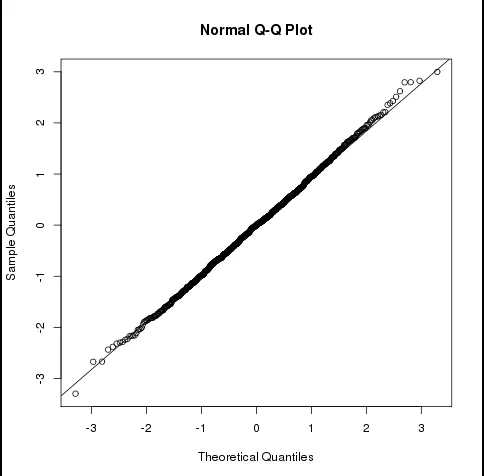
Figure 2.2: Normal Q-Q plot ofT = βb_wnp−β0

b

σ from 1000 simulations under the truncation scenario

for the second model described in Table 2.1 .

Here θ1 = 0.40 andθ2 = 0.25, and n=100. Here _bσis the standard error estimate of βbwnp, and is

estimated using the simple bootstrap method.

2.4. Simulations

In this section we examine the performance of the proposed weighted estimators and compare

them to the na¨ıve unweighted estimator which ignores truncation. In all simulations, the survival

times were generated from a proportional hazards model with hazard functionλ(t|Z) =λ0(t)eβ0Z,

and follow a Weibull distribution with scale parameterρ= 0.1and shape parameterκ= 1.2. We set

β0= 1, and generated the explanatory variableZfrom a Unif[0,1] distribution. We simulated the left

truncation time from ac1Beta(θ1,1) distribution and the right truncation time from ac2Beta(1, θ2)

distribution, with c1 = c2 = 30. We chose these distributions based on our data example. The

assumption of the beta distribution for the truncation times in our data example was validated by a

goodness-of-fit test (Section 2.5).

We conducted 1000 simulation repetitions with sample sizes ofn= 50, 100, and 250. To obtain

nobservations after truncation, we simulatedN = n

truncated data. For each simulation, we estimated the hazard ratio using the na¨ıve unweighted

es-timator which ignores truncation(βbuw), the parametric weighted estimator(βbw

b

θ), the nonparametric

weighted estimator(βbwnp), and the complete case estimator(βbcc)based on the full (truncated and

non-truncated) sample. For these estimators, we calculated the estimated bias (βb−β0), observed

sample standard deviations (SD), estimated standard errors (SEc), and the average empirical

cov-erage probability of the 95% confidence intervals (Cov). We used 2000 bootstrap resamples to

estimate the standard error and confidence interval ofβbwnp.

Table 2.1 shows the results of the simulations described above. In the first model we setθ1= 0.06

andθ2= 0.60, which produced mild left and right truncation and a total of 20% of the observations

truncated. In the second model we setθ1= 0.15andθ2= 1, which produced moderate truncation

from the left and right and a total of 40% of the observations truncated. In the third model we set

θ1= 0.40andθ2= 0.25, which produced heavy left truncation and mild right truncation and a total

of 60% of the observations truncated. In the fourth model we setθ1 = 0.50 andθ2 = 2.5, which

produced both heavy left and right truncation and a total of 80% of the observations truncated.

In all models, the weighted estimatorsβbw

b

θ andβbwnp had little bias, while the unweighted estimator

b

βuw was biased. The observed sample standard deviations of βbw

b

θ corresponded well with the

standard error estimates based on asymptotic theory. The observed sample standard deviations of

b

βwnp were accurately estimated by the bootstrap technique, and were slightly greater than those of

b βw

b

θ. Both weighted estimators had coverage probabilities that were close to the nominal level of

0.95. All of these results held for both smaller (n=50) and larger (n=250) sample sizes. We note

that the high coverage probabilities ofβbuw are an artifact of its large standard error relative to its

bias, which led to wider confidence intervals forβbuw. In simulations where the standard error ofβbuw

was small relative to its bias, the coverage probabilities ofβbuw did not come close to the nominal

level (e.g. Table 2.2).

We now examine the bias of βbwnp and βbuw as a function of left and right truncation proportion

(Figure 2.3). For the purpose of clarity we do not includeβbw

b

θ in Figure 2.3, but note that its bias

was nearly identical to that ofβbwnp. Even under mild truncation, βbuw was biased, and this bias

increased drastically as the proportion of right truncation increased. Here βbwnp had little bias,

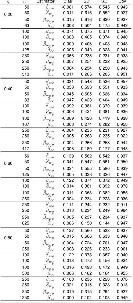
Table 2.1: Simulation results

q n Estimator Bias SD SEc Cov

0.20

50 βbuw -0.081 0.574 0.545 0.943

50 βbw

b

θ -0.011 0.616 0.552 0.927

50 βb_wnp -0.015 0.616 0.620 0.937

63 βbcc 0.003 0.504 0.475 0.943

100 βbuw -0.071 0.375 0.371 0.945

100 βbw

b

θ 0.003 0.405 0.374 0.940

100 βbwnp 0.000 0.406 0.408 0.943

125 βbcc -0.005 0.340 0.328 0.941

250 βbuw -0.066 0.235 0.231 0.938

250 βbw

b

θ 0.007 0.254 0.232 0.925

250 βbwnp 0.004 0.254 0.250 0.945

313 βbcc 0.011 0.205 0.205 0.951

0.40

50 βbuw -0.031 0.548 0.536 0.957

50 βbw

b

θ 0.053 0.593 0.551 0.935

50 βb_wnp 0.045 0.605 0.626 0.934

83 βbcc 0.047 0.423 0.404 0.949

100 βbuw -0.092 0.381 0.370 0.939

100 βbw

b

θ -0.006 0.424 0.381 0.936

100 βbwnp -0.009 0.426 0.419 0.938

167 βbcc 0.008 0.274 0.282 0.958

250 βbuw -0.084 0.235 0.231 0.927

250 βbw

b

θ 0.005 0.263 0.235 0.922

250 βbwnp 0.004 0.266 0.258 0.944

417 βbcc 0.008 0.180 0.177 0.948

0.60

50 βbuw 0.139 0.562 0.542 0.937

50 βbw

b

θ 0.041 0.547 0.561 0.950

50 βbwnp 0.034 0.555 0.580 0.939

125 βbcc 0.005 0.338 0.326 0.947

100 βbuw 0.122 0.374 0.372 0.949

100 βbw

b

θ 0.014 0.361 0.392 0.970

100 βbwnp 0.011 0.363 0.382 0.955

250 βbcc -0.004 0.234 0.228 0.936

250 βbuw 0.111 0.244 0.232 0.911

250 βbw

b

θ 0.013 0.234 0.249 0.964

250 βb_wnp 0.005 0.237 0.234 0.937

625 βbcc 0.006 0.150 0.144 0.947

0.80

50 βbuw -0.127 0.560 0.538 0.937

50 βbw

b

θ -0.015 0.666 0.633 0.940

50 βbwnp -0.004 0.724 0.701 0.947

250 βbcc 0.008 0.226 0.233 0.961

100 βbuw -0.122 0.373 0.367 0.940

100 βbw

b

θ 0.013 0.472 0.456 0.924

100 βb_wnp 0.016 0.493 0.472 0.949

500 βbcc 0.006 0.162 0.164 0.955

250 βbuw -0.163 0.236 0.228 0.878

250 βbw

b

θ -0.021 0.316 0.328 0.913

250 βb_wnp -0.019 0.315 0.294 0.927

1250 βbcc 0.000 0.104 0.103 0.949

qis proportion of truncated observations,nis size of observed sample.βbuwdenotes na¨ıve unweighted estimator,βbw

b

θdenotes proposed

parametric weighted estimator,βbwnpdenotes proposed nonparametric weighted estimator,βbccdenotes unattainable complete case

estimator based on both truncated and non-truncated observations. SD is empirical standard deviation of estimates across simulations,SEc is average of estimated standard errors, Cov is coverage of 95% confidence intervals. True value ofβis 1.

We also examined the robustness ofβbw

b

θ under misspecification of the truncation distribution in

Ta-ble 2.2. In this setting,βbw

b

Figure 2.3: Comparing bias and MSE (mean-squared error) of estimators

Bias of the unweighted estimator βbuw (black) and nonparametric weighted estimator βbwnp (gray).

Left truncation time simulated from ac1Beta(θ1,1)distribution, right truncation time simulated from

ac2Beta(1, θ2)distribution, withc1=c2= 30. Hereθ1ranges from 0.025 to 0.50 which results in a

range of 5% to 65% truncation from the left, andθ2 ranges from 0.25 to 5 which results in a range

of 5% to 45% truncation from the right. The remaining settings are kept the same as in Table 2.1, withn= 250.

assumptions for the truncation times.

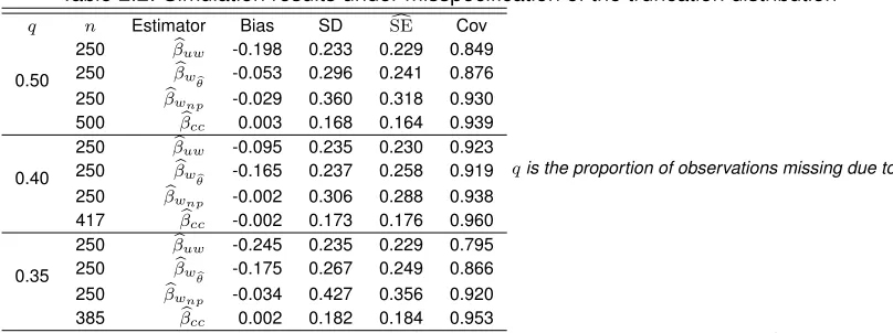
Table 2.2: Simulation results under misspecification of the truncation distribution

q n Estimator Bias SD SEc Cov

0.50

250 βbuw -0.198 0.233 0.229 0.849 250 βbw

b

θ -0.053 0.296 0.241 0.876 250 βbwnp -0.029 0.360 0.318 0.930 500 βbcc 0.003 0.168 0.164 0.939

0.40

250 βbuw -0.095 0.235 0.230 0.923 250 βbw

b

θ -0.165 0.237 0.258 0.919 250 βbwnp -0.002 0.306 0.288 0.938 417 βbcc -0.002 0.173 0.176 0.960

0.35

250 βbuw -0.245 0.235 0.229 0.795 250 βbw

b

θ -0.175 0.267 0.249 0.866 250 βbwnp -0.034 0.427 0.356 0.920 385 βbcc 0.002 0.182 0.184 0.953

qis the proportion of observations missing due to

truncation andnis the size of the observed sample.βbuwdenotes the na¨ıve unweighted estimator,βbw

b

θdenotes the

proposed parametric weighted estimator,βbwnpdenotes the proposed nonparametric weighted estimator, andβbccdenotes

the unattainable complete case estimator based on both truncated and non-truncated observations. SD is the empirical standard deviation of estimates across simulations,SEcis the average of the estimated standard errors, Cov is the

coverage of 95% confidence intervals. The true value ofβis 1.

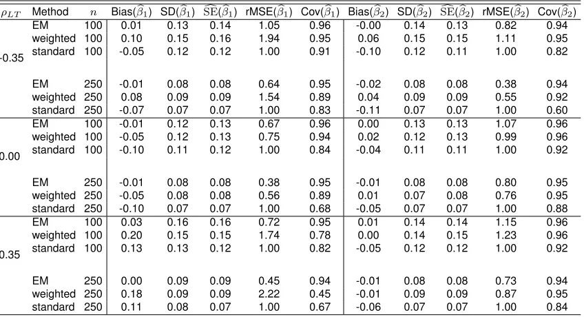
asV =U+d0, whered0can be random or constant. To assess the performance of our proposed

estimators under this dependent truncation structure, we conducted a simulation study in Table 2.3.

The results are similar to those presented in Table 2.1.

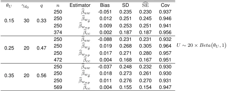
Table 2.3: Simulation results under dependent truncation structureV =U+d0.

θU γd0 q n Estimator Bias SD SEc Cov

0.15 30 0.33

250 βbuw -0.051 0.235 0.230 0.937 250 βbw

b

θ 0.012 0.251 0.245 0.946 250 βbwnp 0.009 0.253 0.251 0.941 374 βbcc 0.002 0.187 0.187 0.956

0.25 20 0.47

250 βbuw -0.088 0.231 0.231 0.932 250 βbw

b

θ 0.019 0.268 0.305 0.964 250 βbwnp 0.017 0.271 0.280 0.957 472 βbcc 0.004 0.168 0.167 0.951

0.35 20 0.56

250 βbuw -0.037 0.248 0.232 0.930 250 βbw

b

θ 0.018 0.273 0.261 0.930 250 βbwnp 0.011 0.276 0.270 0.931 569 βbcc 0.004 0.155 0.154 0.947

U∼20×Beta θU,1

,

d0∼U nif0, γd0

. The remaining settings were kept the same as in the simulations in Section 2.4 of the paper.qis the proportion of observations missing due to truncation andnis the size of the observed sample.βbuwdenotes the na¨ıve

unweighted estimator,βbw

b

θdenotes the proposed parametric weighted estimator,βbwnpdenotes the proposed

nonparametric weighted estimator, andβbccdenotes the unattainable complete case estimator based on both truncated and

non-truncated observations. SD is the empirical standard deviation of estimates across simulations,SEcis the average of

the estimated standard errors, Cov is the coverage of 95% confidence intervals. The true value ofβis 1.

2.5. Application to Alzheimer’s Disease Study

We illustrate our method by considering an autopsy-confirmed AD study conducted by the Center

for Neurodegenerative Disease Research at the University of Pennsylvania. The target population

for the research purposes of this study consists of all subjects with AD symptom onset before

2012 that met the study criteria and therefore would have been eligible to enter the center. Our

observed sample contains all subjects who entered the center between 1995 and 2012, and had

an autopsy performed before 2012. Thus one criterion for a subject to be included in our sample

is that they did not succumb to AD before they entered the study, yielding left truncated data. In

addition, our sample only contains subjects who had an autopsy-confirmed diagnosis of AD, and

therefore we have no knowledge of subjects who live past the end of the study. Thus our data is

also right truncated. Our data consists of n=47 subjects, all of whom have event times. The event

time of interest is the survival time (T) from AD symptom onset. The left truncation time (U) is the

time between the onset of AD symptoms and entry into the study (i.e. initial clinic visit). The right

truncation time (V) is the time between the onset of AD symptoms and the end of the study, which

Our motivation for studying the effect of education on survival in AD is that education serves as

a proxy for cognitive reserve (CR). CR theorizes that individuals develop cognitive strategies and

neuronal connections throughout their lives through experiences such as education and other forms

of mental engagement (Valenzuela and Sachdev, 2007). For example, CR may have a protective

role in the brain, and therefore lengthen survival during the course of the disease (Ientile et al.,

2013). Paradise et al. (2009) and Meng and D’Arcy (2012) failed to detect an effect of education

on survival from AD symptom onset. However the studies included in their meta-analyses did not

consist of populations with autopsy-confirmed AD.

Here we assess the effect of education on survival time in our autopsy-confirmed cohort, where

education is measured by years of schooling. The median years of education in this cohort is 16

years. Comparing the low education group (<16 years) and high education group (≥16 years) on

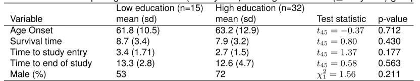
the variables of interest revealed no significant differences (Table 2.4).

Table 2.4: Comparing low education (<16 years) and high education (≥16 years) groups Low education (n=15) High education (n=32)

Variable mean (sd) mean (sd) Test statistic p-value

Age Onset 61.8 (10.5) 63.2 (12.9) t45=−0.37 0.712

Survival time 8.7 (3.4) 7.9 (3.2) t45= 0.80 0.430

Time to study entry 3.4 (1.71) 2.7 (1.5) t45= 1.37 0.177

Time to end of study 13.3 (2.8) 12.6 (4.7) t45= 0.58 0.563

Male (%) 53 72 χ21= 1.56 0.211

Survival time, time to study entry, and time to end of study are measured in years from AD symptom onset.

Since our data is doubly truncated, we apply the Cox regression model using the proposed weighted

estimating equation approach. We check the assumption of independence between the truncation

and survival times in the observable region U ≤ T ≤ V using the conditional Kendall’s tau

pro-posed by Martin and Betensky (2005). The resulting p-value is 0.10, and therefore we do not have

enough evidence to reject the null hypothesis that the observed survival and truncation times are

independent. We justify the identifiability constraints, aHU < aF ≤aHV andbHU ≤bF < bHV, in

Section 2.4.1 below.

We adjust for double truncation using both parametric and nonparametric weights. The parametric

weights are estimated under the assumption that U ∼ c1Beta(α1, β1) and V ∼ c2Beta(α2, β2),

b

α2= 3.0,βb2= 9.7. To check our assumption of the beta distribution, we test the null hypothesisH0:

K(u, v) = Kθ(u, v), whereθ = (α1, β1, α2, β2). Here the parametric joint cumulative distribution

functionKθ(u, v)=Iu/c1(α1, β1)×Iv/c2(α2, β2), whereIx(a, b) =

Rx

0 t

a−1_(1−t)b−1_{dt. As described}

by Moreira, de ˜Una- ´Alvarez, and Van Keilegom (2014), we can testH0using a Kolmogorov-Smirnov

type test statistic Dn = supu,v∈R|Kn(u, v)−Kbθ(u, v)|, where Kn(u, v)is the NPMLE of K(u, v)

(Shen, 2010a). This yields a p-value of 0.60, and therefore we do not have enough evidence

against the beta distribution assumption for the truncation times.

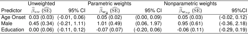
Table 2.5 displays the results from the Cox regression model using no weights, parametric weights,

and nonparametric weights. The effects of age at AD symptom onset and male on survival are

nearly twice as large in the weighted models relative to the unweighted model, but these effects

are only significant under parametric assumptions. When we do not account for double truncation,

there is no effect of education on survival (βbuw = 0; 95% CI: [-0.11,0.12]). When we account for

double truncation, higher education is associated with increased survival under parametric weights

(βwb

b

θ= -0.07; 95% CI: [-0.20,0.06]) and nonparametric weights (βwb np = -0.06; 95% CI: [-0.29,0.19]).

However the confidence intervals for bothβwb

b

θ andβwb np contain 0.

Table 2.5: Application: Education on survival in AD

Unweighted Parametric weights Nonparametric weights

Predictor βbuw(SEc) 95% CI βbw

b

θ(SEc) 95% CI βbwnp (SEc) 95%CI

Age Onset 0.03 (0.03) (-0.01, 0.06) 0.05 (0.02) (0.00, 0.09) 0.05 (0.03) (-0.02, 0.12)

Male 0.45 (0.34) (-0.21, 1.11) 1.01 (0.49) (0.06, 1.97) 0.95 (0.61) (-0.36, 2.18)

Education 0.00 (0.06) (-0.11, 0.12) -0.07 (0.07) (-0.20, 0.06) -0.06 (0.11) (-0.29, 0.19)

2.5.1. Justification of identifiability constraints

Here we justify that the identifiability constraints given in Section 2.2.1, aHU < aF ≤ aHV and

bHU ≤bF < bHV, hold in our data example. First we introduce some notation. Denoteτas the end

of study date,τE as the study entry date, andτAas the date of symptom onset. Note thatτ is the

same for all subjects, whileτEandτAcan differ among subjects. The left truncation time is defined

asU =τE−τA, and the right truncation time is defined asV =τ−τA.

Subjects can theoretically enter the center at the time of AD symptom onset, but not before.

There-fore the smallest possible left truncation time is U=0, and thus aHU = 0. Since recruitment of

subjects into the center stops one week prior to the end of the study, the smallest possible right