Holomorphic Embedding Load Flow Modeling of the Three-phase Active Distribution Network

(1)

Abstract—With large-scale distributed generators (DGs) in an active distribution network (ADN), conventional load flow convergence failure is incurred by heavy power transmission. The Holomorphic Embedding Load Flow Method (HELM) has proven to be more robust than the Newton–Raphson method under heavy power transmission. At present, HELM is mainly designed for balanced transmission networks. In this study, we developed a three-phase HELM model to accommodate DGs, delta connection loads, and ZIP loads for ADN. The effectiveness and better performance of the proposed method under heavy load situations were validated using modified unbalanced IEEE 13, 34, 37, and 123 test feeders.

Index Terms—Active Distribution Network; delta connection; Holomorphic Embedding Load Flow; three-phase

I. INTRODUCTION

OBUST distributed load flow is the cornerstone of active distribution network (ADN) management and control. The Holomorphic Embedding Load Flow Method (HELM) provides a solution to power load flow convergence under heavy power transmission. HELM is non-divergent, which assures its robustness under heavy load scenarios [1] and it is also unsensitive to initial points like the Newton–Raphson method (NR); additionally, in contrast to the NR, it is not sensitive to the initial point. Large-scale distributed generators (DGs) in the distribution network push the ADN load flow close to the divergent region. Hence, a more robust three-phase HELM for ADNs is proposed to cope with this issue.

A. Related Work

HELM, first introduced by A. Trias [1], uses a holomorphic power balanced equation (PBE) to transform the complex node voltage into a function of the node voltage power series with analytic continuation techniques [2][3]. Subramanian et al. [4] extended the PBE for PV nodes with active power constraints, expressed as the summation of two conjugate complex power and voltage magnitude constraints determined by two conjugate complex voltage multiplication. Systematic description and comparisons of HELM and NR are given in [5]. The ZIP load model provides a more accurate feature description of power networks and is derived in detail in [6][7]. Direct current (DC) devices [8], flexible ac transmission system (FACT), and transformer taps [9] can also be modeled using PBEs.

HELM has been implemented in voltage stability analysis [10][11] and nonlinear network reduction [12]. Compared with step-by-step NR-based continuation flow methods, HELM is

capable of calculating the load flow under different load scales simultaneously [13][14], instead of step by step, which speeds up voltage stability. Moreover, the initial point of HELM is not necessarily1 0 , and it is applicable to large-scale transmission networks [15].

B. Main Contribution

The existing model for HELM is applied mainly to balance transmission networks. In this study, to assure HELM application in ADN, three-phase network constraints of the complex node voltage power series for ADN were developed to cope with the delta connection load, ZIP load, and DGs. Phase-to-phase complex voltage variables and additional linear constraints were added in the proposed three-phase HELM model to handle delta connection devices. To improve three-phase HELM efficiency, conventional nonlinear zero-power injection-network constraints are converted to a linear zero-current injection network. Based on this approach, we implemented numerical simulations on modified unbalanced IEEE 13, 34, 37, and 123 test feeders to compare the proposed three-phase HELM with NR and Levenberg–Marquardt (LM) methods.

II. HELM INTRODUCTION

We begin with an introduction of HELM, in which we assume that the complex node voltage can be expressed as a power series of complex number s:

 

 

0 n

n

V s V n s







, (1)

where V n

 

is the Taylor series coefficient and n is the index. The PBE Taylor series generally has the following form:

 







 



 



 







0

1 0

0 0 1

n

F V s G V s

f s f n s

G s g g n s 



   

   

(2)

where f n

 

and g n

 

are Taylor series coefficients and n is the index.

Given that the coefficients on the left and right sides must be equal, new equations for PBE are obtained:

   





 



   



 





0 , 1 , 0 0 0 , 1 , ;

...;

1 ;

f V V f g g V V

f n g n

  

  (3)

Holomorphic Embedding Load Flow Modeling

of the Three-phase Active Distribution Network

Yuntao Ju,

Member, IEEE

R

(2)

where f V



   

0 ,V 1 ,



and g V



   

0 ,V 1 ,



are linear functions of V

   

0 ,V 1 , V n

 

.

Therefore, HELM can be used to solve the PBE with recursive liner equations, as shown in (3), giving

   

0 , 1 ,

V V . The load flow solution is obtained at s1. The complex node voltage at s0 is called the ‘white germ solution,’ which is determined by solving the constraint equations of the linear alternating current (AC) network.

A. Linear Constraints in HELM

Here, we describe the linear constraints of HELM. We assume that the linear constraints for the complex node voltage are given by:

A V b. (4)

According to (1), the above equation can be described using a power series:

 

0 n

n

A V n s b







. (5)

Then the linear constraints of (5) can be transformed into:

 

0 1 0 0 AV b AV AV n         _   

. (6)

HELM can easily accommodate the linear constraints. The slack bus constraints, sequence transform equations, and zero current injection bus are all described by (6). These models will be detailed in Section III.

III. THREE-PHASE ACTIVE DISTRIBUTION NETWORK MODEL

A. Definition of Three-phase Bus and Calculation Node

In three-phase network analysis, each bus will have a one-phase node, two-phase nodes, or three-phase nodes. Herein, for the sake of clarity, a three-phase Bus (TBus) represents a collection of nodes and calculation nodes (CNodes) are the nodes used in three-phase load flow numerical calculations.

B. Y-Connection PQ Load TBus

There are three CNodes for the Y-connection PQ load. It is not difficult to handle each PQ CNode in three-phase HELM. The holomorphic embedding formulation for each CNode is as follows:

 









 





 





2 , , 1

* * * 2

2 ,

0 1 2

j

0 1 2

c c c c

c

N

i n tr n n n

n

i i

i i i

i sh i i i

Y V V s V s

sP Q

W W s W s

sY V V s V s

             



, (7)

where i and n_c denote the CNode index, P_i and Q_i represent

the node injection power, and _,

c

in tr

Y is the CNode admittance matrix without the shunt at CNode i Y_{i sh}_, . W_i*

 

s is defined as:

 

 

* * * * 2

* *

1

0 1 2

i i i i

i

W s W W s W s

V s

     . (8)

Given the germ solution V_i

 

0 , the coefficients in (8) can be calculated by the convolution of W_i*

 

s and Vi*

 

s :

 

  



 

* * 1 * * * * 0

0 1 0 0

0 1

i i

n

i i i i

W V for n

W n W V n V for n

               



. (9)

C. D-Connection PQ Load TBus

Assume that i j k, , is responding to ABC three-phase CNodes in a D-Connection PQ load. To describe the D-connection PQ load between CNodes, phase-to-phase complex voltage is added as an additional variable, with the following linear constraints:

ij i j

jk j k

ki k i

V V V

        _ _ 

. (10)

The linear constraints are easily accommodated by HELM, as discussed in Section IIA.

The D-Connection PQ load branch current will contribute to CNode injections at both terminals. For instance, at CNode i, the holomorphic embedding formulation is given by:

 









 





 





2 , , 1

* * * 2

, , ,

2 ,

0 1 2

j

0 1 2

c c c c

c

N

i n tr n n n

n

ij ij

br ij br ij br ij

i sh i i i

Y V V s V s

sP Q

W W s W s

sY V V s V s

              



, (11)

where

 

 

* * * * 2

, _* _* , , ,

1

0 1 2

br ij br ij br ij br ij

ij

W s W W s W s

V s

     .

At CNode j, the holomorphic embedding formulation is expressed as:

 









 





 





2 , 1

* * * 2

, , ,

2 ,

0 1 2

j

0 1 2

c c c c

c

N

jn tr n n n

n

ij ij

br ij br ij br ij

j sh j j j

Y V V s V s

sP Q

W W s W s

sY V V s V s

             



. (12)

D. Distributed Generators Model

(3)

photovoltaic generators are mainly considered. dg Z i j k

Fig. 1. Simple illustration of distributed generators (DGs).

The power electronic-interfaced generators can be modelled with a current or voltage source behind impedance Z_dg, as shown in Fig. 1. There are mainly two kinds of control modes for the three-phase converter [16]: balanced internal voltage

i

V  V ej j120 

j120 k

V e 

 and balanced injection current i

I  I ej j120 

j120 k

I e 

 .

1) Balanced internal voltage without voltage control

For this kind of DG, there are two linear voltage constraints: j120

j120

i j

i k

V V e

         

. (13)

The three-phase total active and reactive powers are known. Thus, the holomorphic embedding formulation is given by:

 





 





 









 





 





 





2 , , 1 -j120 2 , , 1 j120 2 , , 1

* * * 2

2 ,

-j120 2

,

0 1 2

j

0 1 2

c c c c

c

c c c c

c

c c c c

c

N

i n tr n n n

n

N

j n tr n n n

n

N

k n tr n n n

n

dg dg

i i i

i sh i i i

j sh j j j

Y V V s V s

e Y V V s V s

sP Q

W W s W s

sY V V s V s

se Y V V s V s

se                                



 





j120 2

, 0 1 2

j sh j j j

Y V V s V s



  

. (14)

where P_dg,Q_dg corresponds to the total active and reactive power.

2) Balanced internal voltage with voltage control

For this kind of DG, apart from the two linear voltage constraints, there is an additional holomorphic embedding formulation for voltage magnitude V_i control:

 

 

  



2

1 *

,re 0 1

1 1 ₁

2 2

sp _n

i

i n n i i

V

V n V V n



    





  



 , (15)

where subscript re denotes the real part of the complex number, sp

i

V is the voltage magnitude control targets, and



_ni is the Kronecker delta function:

1 0

ni

if i n otherwise

   

 . (16)

A detailed derivation of (15) can found in [5].

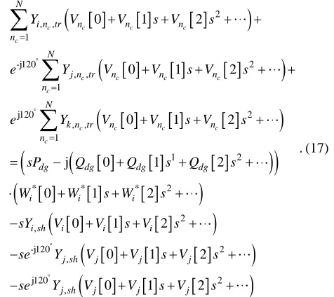
The total reactive power for the DGs will be unknown. The holomorphic embedding formulation is written as:

 





 





 





 









 





 





2 , , 1 -j120 2 , , 1 j120 2 , , 1 1 2

* * * 2

2 ,

-j120 ,

0 1 2

j 0 1 2

0 1 2

c c c c

c

c c c c

c

c c c c

c

N

i n tr n n n

n

N

j n tr n n n

n

N

k n tr n n n

n

dg dg dg dg

i i i

i sh i i i

j sh j

Y V V s V s

e Y V V s V s

sP Q Q s Q s

W W s W s

sY V V s V s

se Y V

                              



 





 





2 j120 2 ,

0 1 2

j j

j sh j j j

V s V s

se Y V V s V s

  

   

. (17)

Multiplication of two power series can be described with convolution; as such, the coefficients in the above equations can be converted to the following:

 





 

















j120 , , 1 1 j120 , 1 1 * * 1

, , 1 , 1

1 j *

1 1 1

c c c c

c c

c c c

N N

i n n j n n

n n

N

k n n n

n

dg i dg dg i

i sh i j n i k n k

Y V n e Y V n

e Y V n

P W n Q n Conv Q W

Y V n Y V n Y V n

                 _  _        



_{, (18)}

where





1 * 1 * n dg i

Conv Q W



denotes the convolution of the two power series.

3) Balanced injection current

For this kind of DG, the injection current power for CNode

, ,

i j k I_i, I_j,I_k are added as unknowns. The power series is given by:

 

 

0 n i i n

I s I n s







. (19)

The linear constraints for injection current are as follows: j120

j120

i j

i k

I I e

         

. (20)

(4)

 

 





 











 



*

* *

2

j120 2

* * * 2

0 1 2

j 0 1 2

i i j j k k

i i i

j j j

k k k

dg dg i i i

V I V I V I

V V s V s

e V V s V s

sP Q D D s D s





 

  

   

     

(21)

where:

 

 

* * * * 2

* *

1

0 1 2

i i i i

i

D s I I s I s

I s

     . (22)

E. ZIP Load

The current component in ZIP load is of utmost important in the holomorphic embedding formulation. The constant impedance and constant power parts of the ZIP load are represented, respectively, as a linear impedance branch and PQ load with respect to the CNode voltage (for the Y-connection or with respect to the phase-to-phase voltage for the D-connection branch).

For the Y-connection current component, the load can be described as:

, 0 , 0

i p I i q I i

S a P V ja Q V (23)

According to the derivation in [6], the coefficient power series of the injection current is given by:

   







  



  

2 _*

, 0 , 0

0 1

1 2 0

n

i p I q I i

j

n

j

I n I a P ja Q V n j W j

I n j I j

 



   

 



.(24)

Similarly, a derivation can be implemented for the D-connection current component with respect to the phase-to-phase branch current I_ij.

F. Zero-injection CNode

Unlike the existing HELM, the zero-injection constraints can be written in terms of the linear constraints in the proposed model:

, 1

0

c c c

N

i n n n

Y V





. (25)

As described in Section IIA, HELM can easily accommodate linear constraints. With (25), for example, ADNs with a large-scale zero-injection CNode can be solved more effectively.

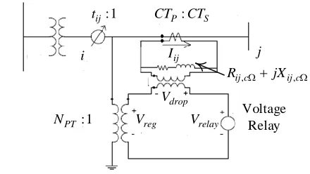
G. Step Voltage Regulator

A step voltage regulator (SVR) is widely applied in ADNs, as illustrated in Fig. 2. The line voltage drop compensator is coupled to the distribution line through a voltage transformer (turns ratio N_PT:1) and a current transformer (turns ratio

:

P s

CT CT ). The impedance of the compensator represents the equivalent impedance from the regulator to the load center. The

relay voltage is given by:



, j ,



relay reg drop reg ij c ij c ij

V V V V  R _ X _ I , (26) where R_{ij c}_,jX_{ij c}_, denotes compensator impedance in

ohms, V_reg is the voltage at voltage transformer secondary side, and V_drop is the voltage drop along the equivalent compensator impedance with line current I_ij.

Similar to the load flow calculation procedure in [17] and [18], the tap calculation of the SVR tap round



V_relayVsp 0.75



is updated after obtaining the flow solution. Herein, round means to round to an integer number.

i j

:1 PT

N

:

P S

CT CT

Voltage Relay :1

ij

t

ij

I

, ,

ij c ij c

R _ jX _

drop

V

reg

V V_relay

Fig. 2. Step voltage regulator (SVR) with line drop compensator.

In conventional ladder iterative load flow, the SVR is modelled as an ideal transformer. However, in three-phase HELM, the SVR is modelled as an ideal transformer with a very small impedance. This has little impact on the three-phase HELM results, while ensuring that the SVR can be incorporated easily into the admittance matrix. This approach is also used in the implicit Z_bus method of OpenDSS [18].

H. Floating point network

Floating point network problem will be posed for active distribution network of Delta connection with no reference CNode. To cope with this issue, the zero sequence reference constraints for three-phase abc CNode (i j k, , ) will be added.

0

i j k

VV V  (27)

(27) is linear constraints and can be handled according to Section IIA.

IV. FLOWCHART OF THE PROPOSED THREE-PHASE HELM The steps for the proposed three-phase HELM are given below.

Step 1: Calculate the complex voltage V_i

 

0 , complex phase-to-phase voltage V_ij

 

0 , complex injection current

 

0

i

I (for DGs), and complex phase-to-phase current

 

0

ij

(5)

Step 2: For the m step, according to proposed power series expression (7)(11)(14)(15)(17)(21)(24), calculate

 

i

V m ,V m_ij

 

,I m_i

 

,Iij

 

m .

Step 3: Compare the power mismatch with the small convergence criterion; if satisfied, go to Step 4. If oscillation occurs, then stop (failure). Otherwise, go to Step 2.

Step 4: Check the SVR for a voltage limit violation. If a violation has occurred, update the SVR tap and return to Step 1 to update the admittance matrix.

Step 5: Calculate all variables using

     

0 1 2

xx x x  .

Note that for HELM, oscillation of the solution means that the load flow cannot be solved.

V. NUMERICAL TESTS

The proposed three-phase HELM was implemented on modified IEEE 13, 34, 37, and 123 test feeders with DGs. Table I lists the arrangement of the DGs for each case. The positive and negative sequence impedance of each three-phase DG was 0.00254 p.u., and the zero-sequence impedance of each DG was 0.004 p.u. The specified complex power for the three-phase DG was 0.008 + 1j * 0.008 p.u., and the base power was 1 MVA. All computations were carried out with MATLAB on an Intel (R) Core (TM) E5-2630 central processing unit (CPU) with 2.2 GHz and 128 GB RAM.

TABLE I

DGARRANGEMENT AND PARAMETERS

Case name Bus no. with three-phase DG

For voltage control, specified voltage

magnitude IEEE 13 634, 675, 670 0.971, 0.962, 0.973 IEEE 34 802, 848, 836 1.049, 1.1, 1.099 IEEE 37 740, 725, 731 0.908,0.920, 0.915 IEEE 123 89.87, 91 1.020, 1.02, 1.02

A. Threephase HELM in Comparison with Conventional NR

and Levenberg–Marquardt Load Flows

In the proposed three-phase HELM, NR method, and LM method, N_HELMdenotes the number of terms in the power series utilized in HELM; N_NR and N_LM denote the numbers of iterations taken by the NR and LM methods, respectively.

HELM

t ,t_NR,t_LM , denote the execution time of three-phase HELM, NR, and LM. M_HELM, M_HELM ,M_HELMdenote the mismatch of three-phase HELM, NR, and LM.

The test case IEEE 13H denotes a heavy load situation with all loads multiplied by 2.3.

TABLE II

THREE-PHASE HELMIN COMPARISON TO NR AND LM

Case name NHELM NLM NNR MHELM MLM

IEEE 13 30 13 4 8.5E-6 1.5E-10

IEEE 34 30 25 3 7.7E-6 1.5E-3

IEEE 37 30 13 3 1.2E-6 7.1E-10

IEEE 123 30 25 3 2.0E-6 5.8E-3

IEEE 13H 30 25 - 9.3E-6 4.2E-3

Case name MNR tHELM(

s) LM

t (s) tNR(s)

IEEE 13 1.3E-13 0.141 0.087 0.005 IEEE 34 1.8E-11 0.57 0.151 0.008 IEEE 37 4.7E-12 0.483 0.1047 0.0065 IEEE 123 8.2E-10 1.016 0.233 0.076

IEEE 13H - 0.146 0.121 -

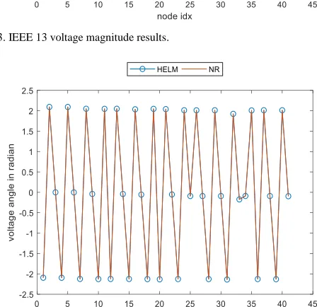
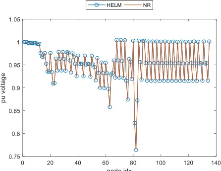
As illustrated in Table II, a comparison of three-phase HELM with robust LM shows that both can obtain a solution under a heavy load; however, HELM provided more stable results than LM, with LM showing a large mismatch. Comparing three-phase HELM and NR, NR obtained the most accurate results and was faster than HELM and LM; however, NR was not robust under a heavy load. We were unable to determine the execution time of three-phase HELM, as it requires additional study, e.g., zero-injection CNode modeling. Figures 3–10 show the load flow results of HELM and NR; the voltage magnitude and angle calculations were in good agreement. In summary, three-phase HELM is promising for ADN analysis.

Fig. 3. IEEE 13 voltage magnitude results.

(6)

Fig. 6. IEEE 34 voltage angle results.

B. Comparison between Linear Current Constraints and Nonlinear Zero PQ Constraints for Zero-Injection CNode

(7)

methods, we let N_zero denote the zero-injection CNode percentage in ADNs, t_NL the CPU time of HELM with nonlinear zero injection power constraints, and t_L the CPU

time of HELM with linear zero-injection power constraints. As shown in Table III, the zero-injection CNode percentages in the ADNs were large. We expect HELM performance to improve significantly with linear zero-injection current constraints.

TABLE III

THREE-PHASE HELMIN COMPARISON TO NR AND LM

Case name Nzero% tL tNL

IEEE 13 58.54 0.34

IEEE 34 64.44 0.36

IEEE 37 73.68 0.42

IEEE 123 66.44 0.38

VI. CONCLUSION

HELM was applied to ADN network load flow analysis. Coping with the three-phase features of the delta-connection load, DGs are of fundamental importance for three-phase network analysis.

The linear zero-injection current holomorphic embedding formulation proposed in this paper can improve the three-phase HELM.

VII. ACKNOWLEDGMENT

This work was supported in part by the National Natural Science Foundation of China (Grant No.51707196).

REFERENCES

[1] A. Trias, “The Holomorphic Embedding Load Flow Method,” in 2012 IEEE Power and Energy Society General Meeting, 2012, pp. 1–8. [2] H. Stahl, “On the convergence of generalized Padé approximants,”

Constr. Approx., vol. 5, no. 1, pp. 221–240, Dec. 1989.

[3] H. Stahl, “The convergence of Padé approximants to functions with branch points,” J. Approx. Theory, vol. 91, no. 2, pp. 139–204, Nov. 1997. [4] M. K. Subramanian, Y. Feng, and D. Tylavsky, “PV bus modeling in a

holomorphically embedded power-flow formulation,” in 2013 North American Power Symposium (NAPS), 2013, pp. 1–6.

[5] S. Rao, Y. Feng, D. J. Tylavsky, and M. K. Subramanian, “The holomorphic embedding method applied to the power-flow problem,” IEEE Trans. Power Syst., vol. 31, no. 5, pp. 3816–3828, Sep. 2016. [6] S. S. Baghsorkhi and S. P. Suetin, “Embedding AC Power Flow in the

Complex Plane Part I: Modelling and Mathematical Foundation,” Mar. 2016.

[7] S. S. Baghsorkhi and S. P. Suetin, “Embedding AC power flow in the complex plane part II: A reliable framework for voltage collapse analysis,” Sep. 2016.

[8] A. Trias and J. L. Marin, “The Holomorphic Embedding Loadflow Method for DC Power Systems and Nonlinear DC Circuits,” IEEE Trans. Circuits Syst. I Regul. Pap., vol. 63, no. 2, pp. 322–333, Feb. 2016. [9] M. Basiri-Kejani and E. Gholipour, “Holomorphic embedding load-flow

modeling of thyristor-based FACTS controllers,” IEEE Trans. Power Syst., vol. 32, no. 6, pp. 4871–4879, Nov. 2017.

[10] S. D. Rao, D. J. Tylavsky, and Y. Feng, “Estimating the saddle-node bifurcation point of static power systems using the holomorphic embedding method,” Int. J. Electr. Power Energy Syst., vol. 84, pp. 1–12, Jan. 2017.

[11] C. Liu, B. Wang, F. Hu, K. Sun, and C. L. Bak, “Online voltage stability assessment for load areas based on the holomorphic embedding method,” IEEE Trans. Power Syst., pp. 1–1, 2017.

[12] S. Rao and D. Tylavsky, “Nonlinear network reduction for distribution networks using the holomorphic embedding method,” in 2016 North American Power Symposium (NAPS), 2016, pp. 1–6.

[13] Y. Zhu and D. Tylavsky, “Bivariate holomorphic embedding applied to the power flow problem,” in 2016 North American Power Symposium (NAPS), 2016, pp. 1–6.

[14] C. Liu, B. Wang, X. Xu, K. Sun, D. Shi, and C. L. Bak, “A

multi-dimensional holomorphic embedding method to solve AC power plows,” IEEE Access, vol. 5, pp. 25270–25285, 2017.

[15] H.-D. Chiang, T. Wang, and H. Sheng, “A novel fast and flexible holomorphic embedding method for power flow problems,” IEEE Trans. Power Syst., pp. 1–1, 2017.

[16] M. Z. Kamh and R. Iravani, “Unbalanced model and power-flow analysis of microgrids and active distribution systems,” IEEE Trans. Power Deliv., vol. 25, no. 4, pp. 2851–2858, Oct. 2010.

[17] W. H. Kersting, Distribution System Modeling and Analysis. Taylor & Francis, 2012.

[18] R. C. Dugan and T. E. McDermott, “An open source platform for collaborating on smart grid research,” in 2011 IEEE Power and Energy Society General Meeting, 2011, pp. 1–7.

The English in this document has been checked by at

least two professional editors, both native speakers

of English. For a certificate, please see:

Creative Commons CC BY