Macro Stress Testing in the Banking System of China
Bo Jiang
received his PhD in Economics from the Nottingham Business School, Nottingham
Trent University in 2015. His research work has focused on financial stability, both in
the UK and in the China. His research uses econometrics analysis of time series data
and panel data.
Bruce Philp
is presently the Head of Research and Enterprise at Birmingham City University
Business School. He obtained his PhD from the University of Manchester in 2001 and
since then has published in a number of academic journals, principally in the
macroeconomic study of income distribution and crisis. He is an editorial board
member for Review of Political Economy, and Economic Issues.
Zhongmin Wu
2
Journals such as Economics Letters, Industrial Relations Journal, Journal of
Development Studies, Regional Studies, Applied Economics, China Economic Review,
Journal of Economic Studies, North American Journal of Economics and Finance, etc.
He edited two books, both published by Routledge in 2009.
Correspondence
: Dr Zhongmin Wu, Nottingham Trent University, 50 Shakespeare
Street, Nottingham NG1 4FQ, UK
ABSTRACT
3
JEL CODES: C15; E58; E44; G21
KEY WORDS: China; Macro stress testing; Non-performing loan; VAR analysis
1. INTRODUCTION
In recent years banks have engaged in increasingly complex and diverse international financial
activities. The role of banks, as one of the most important financial intermediaries in an
economy, and as a prerequisite for sustainable economic growth, reinforces the fact that
instability in the banking system would be costly for the real economy. This is manifest by the
myriad ways the current Global Financial Crisis (GFC) has impacted economies (e.g.
Tagkalakis, 2013; Aboody et al., 2014).1,2 In particular, the costs and losses, at the national
level, associated with failures within the banking system, underscore the need for supervision
with a macro-prudential perspective, particularly with regard to how banks measure and control
their risk exposure.
From the macro-prudential perspective, the Basel III Accord emphasized the need for the
development of a more robust stress-testing approach compared to Basel II.3-6 The emphasis
suggests that up-to-date risk management techniques —particularly, ‘macro stress-testing’ —
have become effective tools in assessing stability of the banking system, and the financial
4 banks, where stress tests are a prudent technique alongside the traditional regulation methods
used to assess risk exposure in the financial system (Marcelo et al., 2008).8
In this paper we focus on macro stress testing in assessing financial stability in China, and
we address two questions that naturally arise. First, how should we measure the potential risks
in the banking system? Secondly, how do we quantify the vulnerability of the banking system
to potential risks? To achieve answers to these, we develop a framework for macro stress testing
of credit exposures in the Chinese banking system. Our empirical analysis adopts a vector
autoregression (VAR) approach, and investigates the relationship between the ratio of
non-performing bank loans and key macroeconomic factors, such as GDP growth, RPI, the
unemployment rate, fixed investment, real estate price indexes, the money supply, interest rates,
and the exchange rate. Macro stress testing assesses the credit risk of banks’ overall loan
portfolios and mortgage exposures by mapping multivariate scenarios against potential risks.
The test introduces different types of macroeconomic shocks into the scenarios, which are
designed to replicate those that have occurred in past financial crises and stochastic simulations.
The present study is thus predicated on the following: first, stress-testing has become an
integral part of banks’ risk management assessments; second, in interpreting the results of stress
tests, many banks create a link between market shocks and banks’ responses. Interestingly, in
China, which is an emergent global economy, stress testing is still at the embryonic stage. On
this basis, we posit that the analysis contained herein is timely and contributes to our
5
2. BACKGROUND
Previous literature and the experience of the GFC has shown that many financial institutions
can experience large losses. Stulz (2008)9 argues that a large loss is not necessarily a
consequence of risk-management failure, because large losses can happen even if risk
management is stringent. In other words, the common task of daily risk management cannot
completely rule out extreme exposure to losses. This notwithstanding, the recent GFC has also
highlighted serious deficiencies in traditional risk management models (e.g. Huang et al., 2009;
Aizenman et al., 2012)10,11 and underscores the necessity for improvements in risk management
systems, and the adoption of improved risk-management measures to better depict the possible
risks. This is why stress tests and scenario analysis are apposite.
Moreover, regulators need to provide a clearer definition of financial stability and the
framework to achieve this goal. Recently, regulators have charged banks with the responsibility
of ensuring a sound, stable and efficient banking system as a whole, i.e. financial stability, rather
than only assuring the soundness of their own bank (Borio, 2006).12 Financial stability depends,
in essence, on the prudential regulation and effective supervision which was instituted in 1999
by the IMF and the World Bank via the Financial Sector Assessment Program (FSAP).
Although there is no single generally accepted definition of financial stability, Marcelo et al. suggest that ‘for a given economy, [financial stability] provides sufficient assurance that the
6 between investors and savers) will not be significantly affected by adverse events (shocks)’
(2008, p.65).8 Given the huge negative implications for the real economy in the event of
financial instability, regulatory authorities should have a particular and well-justified interest in
ensuring financial stability (as highlighted by the Basel III Accord).
As a result of the widespread implementation of the FSAP, stress tests are now broadly
utilized. According to Borio et al. (2012),13 micro and macro stress tests have four elements:
the risk exposures subjected to stress; the scenario defining the shocks; the model mapping the
shocks onto an outcome; and, the measure of the outcome. More specifically, the aim of stress
testing is to measure the impact of severe shocks which are potentially able to harm financial
stability. Hence, the results of stress testing are threefold: to add value to the internal control
exercised by banks in the course of risk management; to serve as a basis for fostering prudential
techniques of protection against adverse situations; and, to facilitate prevention, early warning
and response tasks to deal with these adverse situations (see Marcelo et al. 2008).8
As pointed out by Drehmann (2005),14 stress testing models differ in terms of complexity
and the risks considered. Despite many significant contributions to stress testing (e.g.: Elsinger
et al., 2006; Jacobson et al.,2005; De Graeve et al., 2008; Pesaranet al.,2009; Aikman et al.,
2009),15-19 there is no consensus on the set of tools, or the best approach, to use. As a
consequence of this various approaches have been proposed, including Wilson (1997a,
1997b),20,21 Virolainen (2004),22 Sorge and Virolainen (2006),23 Misina et al. (2006),24 and
7 linear relationship between macroeconomic variables and the probability of default on the
bank’s loan portfolio.
Studies specific to China are sparser. Xu and Liu (2008)26 compare several popular macro
stress testing approaches and focus on the use of macro stress testing to estimate the stability
of the financial system. Using a logit model, Ren and Sun (2007)27 estimate credit risk in the
banking industry. For their part, Chen and Wu (2004)28 empirically investigate vulnerability of
China’s banking system over the period 1978-2000. They uncover evidence to suggest that
macroeconomic dynamics affect the bank’s stability via macroeconomic policies.
3. METHODOLOGY
In testing credit risk exposure in China’s banking system, we will begin by adopting the
framework proposed by Wilson (1997a, 1997b),20,21 Boss (2002)29 and Virolainen (2004)22, i.e.
estimating the relationship between credit risk and macroeconomic dynamics. Next, we employ
the Monte Carlo simulation approach to examine the distribution of possible default rates for
the scenario under investigation.
We define 𝑁𝑃𝐿𝑅𝑡 as the aggregate non-performing loan ratio of the whole banking
system in China in period t. Since 0 ≤ 𝑁𝑃𝐿𝑅𝑡 ≤ 1 we can employ its logit-transformed value
(𝑦𝑡) instead of 𝑝𝑡 as the dependent variable.That is
𝑦 𝑡 = 𝑙𝑛 {
1 − 𝑁𝑃𝐿𝑅𝑡
𝑁𝑃𝐿𝑅𝑡
8 After this canonical processing for the credit risk index (note here that –∞ <𝑦𝑡< +∞), it follows
that the 𝑁𝑃𝐿𝑅𝑡is negatively related to 𝑦𝑡, which means a higher 𝑦𝑡 indicates a better
credit-risk status, and vice versa. Further, preliminary (augmented Dickey-Fuller) unit-root tests with
the time trend and the intercept finds 𝑦𝑡(our dependent variable) to be stationary. More
specifically, 𝑦𝑡 dependents on its lags, and the n lagged values of the macroeconomic
variables:
𝑦𝑡= α + 𝐴1𝑥𝑡−1··· +𝐴𝑛𝑥𝑡−𝑛+ 𝐵1𝑦𝑡−1··· +𝐵𝑛𝑦𝑡−𝑛+ ѵ𝑡 (1)
where 𝑦𝑡 is a vector of endogenous variables and 𝑥𝑡 is a vector of exogenous variables. In this
equation α is the vector of intercepts and 𝐴1··· 𝐴𝑛 are matrices of coefficients on the
macro-economic variable lagged 𝑛 times. The matrices of coefficients 𝐵1··· 𝐵𝑛 are associated with
the lags on the dependent variable, and the disturbance term is given by ѵ𝑡, which may be
contemporaneously correlated but are uncorrelated with their own lagged values and
uncorrelated with all of the right-hand side variables.
This macro-economic framework examines the dynamics of the macro-economic variables
as well. Based on Wilson’s original specification, which every macro-economic variable
follows an autoregressive (AR) process, we generalize a more realistic dynamic process by
adopting by the following specification:
𝑥𝑡= β + 𝐶1𝑥𝑡−1··· +𝐶𝑛𝑥𝑡−𝑛+ 𝐷1𝑦𝑡−1··· +𝐷𝑛𝑦𝑡−𝑛+ 𝜀𝑡 (2)
where β is the vector of intercepts; 𝐶1··· 𝐶𝑛 and 𝐷1··· 𝐷𝑛 are coefficient matrices; and 𝜀𝑡
9 variables are mutually interdependent and equation (4.2) explicitly accounts for feedback
effects of bank performances on the economy (the terms 𝐷1𝑦𝑡−1··· +𝐷𝑛𝑦𝑡−𝑛
).
Equation (4.1)and (4.2) together compose the framework to study the economic performance and the
associated financial stability indicators.
In developing our model we aim to improve on the specification employed in Virolainen
(2004)22 and Wilson 1997a, 1997b).20,21 First, we employ a lag-effect of the macroeconomic
variables to banks’ credit risk. Second, by allowing 𝑥𝑡to depend on 𝑦𝑡−1, 𝑦𝑡−𝑠 this implies
previous bank performances can influence the present macro economy.
Subsequently, we employ Monte Carlo simulations to generate the distribution of possible
credit losses under the macroeconomic shock scenarios, which we can then compare with
possible credit losses under the baseline scenario. Nevertheless, it is instructive to note that this
approach has some limitations, such as the treatment of the contagion effect within the banking
system. First, it is not unusual for central banks to use aggregate data when testing the change
of credit risk in the regional banking system, based on the assumption that we move from top
to bottom. However, the use of aggregate data when assessing credit risk in the whole banking
system is equivalent to conducting micro stress testing with the aggregate data, and ignoring
the structural problems within the financial system. Second, the adaptive response of banking
institutions may generate a feedback effect. It is commonplace that in a number of the macro
stress testing practices the initial shock effect from the macro economy to the banking system
10 of stress testing is prolonged. In other words, the change of risk factors in the first round should
not be treated as the ultimate outcome and underscores the need to continually reassess the
response behavior of the banking system to a (macroeconomic) shock.
4. EMPIRICAL RESULTS AND DISCUSSION
4.1. Variables description and data sources
Following the framework discussed above, we adopt a macroeconomic credit risk model to
estimate the relationship between macroeconomic variables and the non-performing loan ratio
(NPLR) of the banking system covering the period from 2000Q1 to 2012Q3. Due to the
importance of selecting the appropriate variables, Table 1 presents a brief summary of the
variables considered in previous research, which then informs our choice of variables for China.
Based on the aims of this research (and the reliability and availability of data), we will focus
on eight major explanatory variables for China (see Table 2).
Table 1: Summary of Macroeconomic variables employed in previous research
Author(s) Geographical
Location
Macro variables
Wong et al. (2006)30 Hong Kong Real GDP growth; Real GDP growth of Mainland
11 prices.
Bardsen et al.
(2006)31
Norway Real GDP; Real household consumption;
Unemployment; Consumer prices; Interest rate; House
prices.
Bunn et al. (2005)32 United Kingdom Interest rate; GDP; Output gap; Unemployment rate;
Real exchange rate; Inflation rate; House price inflation
rate.
Misina et al. (2006)24 Canada GDP growth rate; Unemployment rate; Interest rate;
Credit/GDP ratio.
Virolainen (2004)22 Finland Nominal GDP growth; Interest rate; Exchange rate;
M2; International balance of payment; Asset price.
We identify three popular dependent variables typically considered in previous research,
namely: the firm’s probabilities of default (PD) (see for example, Pesaran et al., 2006);33
corporate expected default frequencies (EDF) (see for example, Alves, 2005);34 and, the balance
sheet information of the bank (such as NPLR, capital adequacy ratios and liquidity). Compared
to PD and EDFs, balance sheet information is a traditional measurement, but it is limited
because balance sheet information is only available on a relatively low-frequency basis
12 they can be forward-looking. Due to the nature of China’s commercial banks, and the
availability of relevant data, we employ NPLR as the measurable dependent variable pertaining
to the balance sheet. According to the Loan Quality Assessment Guidelines (China Bank
Regulatory Commission, 2005),35 the NPLR is classified as the total of sub-loans,
doubtful-loans and loss-doubtful-loans divided by total doubtful-loans. In other words, a higher NPLR implies a higher
level of credit exposure.
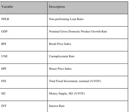
Table 2: Variable list
Variable Description
NPLR Non-performing Loan Ratio
GDP Nominal Gross Domestic Product Growth Rate
RPI Retail Price Index
UNE Unemployment Rate
HPI House Price Index
FIX Total Fixed Investment, nominal (%YOY)
M2 Money Supply, M2 (%YOY)
13
EX Exchange rate, Chinese Yuan to US Dollar
The eight explanatory macroeconomic variables (Table 2), including the GDP growth rate,
the retail price index, the unemployment rate, a house price index, the money supply (M2), the
interest rate, exchange rate, and total fixed investment, can be placed into four categories to
capture different kinds of potential shocks:
1. The business cycle is measured by GDP growth, retail price index (for inflation), and
the unemployment rate, as the stability of the macro-economy is the goal of a healthy
financial system. A growing economy is likely to be associated with rising incomes
and reduced financial distress. Therefore, GDP growth is negatively associated with
the NPLR and unemployment is positively related with the NPLR. After maintaining
high-growth for a number of years, the growth of China’s economy has slowed down
somewhat, while inflation remains above the Government’s target. Thus,
policy-makers in China have been concerned with how to implement a successful
“soft-landing”, whilst dealing with inflation.
2. Credit risk is measured by the interest rate, money supply (M2), and total fixed
investment. Banks are still the major source of corporate and fixed investment in China,
and the interest rate and credit quota have a direct impact on the credit exposure of the
banks’ balance sheets. Otherwise, unlike their counterparts in developed countries,
14 commercial banks in China. A hike in interest rates weakens borrowers’ debt servicing
capacity, thus, NPLR is expected to be positively related with the interest rate.
3. Property-value bubbles, which are measured by house price indexes, have triggered
several financial crises, such as the Florida property bubble in late 1920s (White,
2009),36 the depression of Japan since 1991 (Posen, 2003),37 and the subprime lending
crisis since March 2008. In China, the loans to the real estate sector have grown to
RMB 11.74 trillion in September 2012, an increase of approximately 12.1% since the
end of 2011 (Source: China Banking Regulatory Commission). Should this indicate a
bubble this may create problems since real estate is a major item of collateral, and
banks would be unwilling to service the debt should the value of real estate decline.
4. Exchange rate risk is measured by the exchange rate (Chinese Yuan to US Dollar),
which reflects the global macroeconomic environment. The fluctuation of the
exchange rate might significantly affect the stability of the whole economy and output.
An appreciation of the exchange rate can have mixed implications. On the one hand,
it could weaken the competitiveness of export-oriented firms and adversely affect their
ability to service their debt. On the other, it can improve the debt-servicing capacity of
borrowers who borrow in foreign currency. The sign of the relationship between NEER
and NPL is indeterminate.
These variables are initially chosen as macroeconomic factors by the R-squared values of the
15 index, producer price index, and stock market index, but find no additional explanatory power.
We source the NPLR data from the China Banking Regulatory Commission website and
the Ruisi Statistical database. Other data used in this study are sourced from DataStream, the
National Bureau of Statistics of China, and The People’s Bank of China. The summary
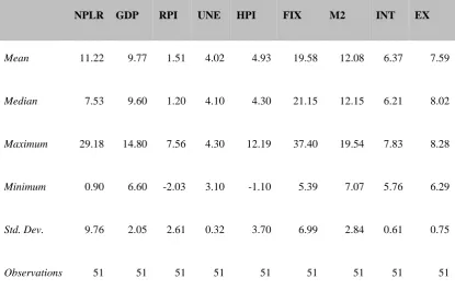
descriptive statistics of data are presented in Table 3.
Table 3: Summary statistics, 2000Q1-2012Q3
Prior to 2000 annual data was only available for some variables. The trend in the NPLR of
the banking system in China had climbed to a peak in 1999, thereafter exhibiting a steady
decline. In part this turning point may be explained by the establishment of an asset
NPLR GDP RPI UNE HPI FIX M2 INT EX
Mean 11.22 9.77 1.51 4.02 4.93 19.58 12.08 6.37 7.59
Median 7.53 9.60 1.20 4.10 4.30 21.15 12.15 6.21 8.02
Maximum 29.18 14.80 7.56 4.30 12.19 37.40 19.54 7.83 8.28
Minimum 0.90 6.60 -2.03 3.10 -1.10 5.39 7.07 5.76 6.29
Std. Dev. 9.76 2.05 2.61 0.32 3.70 6.99 2.84 0.61 0.75
16 management corporation between 1999 and 2004, which was responsible for managing the bad
assets of the four major state-owned commercial banks. Since these “big four” retained in
excess of 60% of the total assets in the whole banking system, the concurrent injection by the
Central Bank of a large amount of funds into these “big four” led to the overall NPLR dropping
significantly.
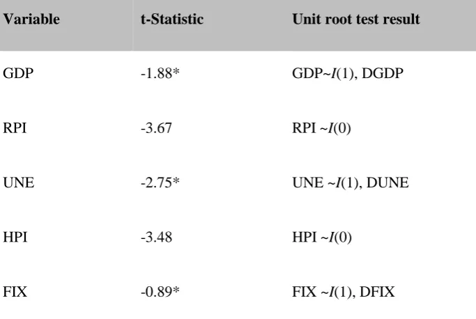
Results of our preliminary tests using the augmented Dickey-Fuller (ADF) method (with
trends and intercepts, testing the time series properties for all these variables) suggest that three
of the macroeconomic series — specifically RPI, HPI, and M2— are stationary I(0). The other five variables — i.e. GDP, INT, EX, UNE and FIX — are first order stationary I(1). Because
of this we use their first differences, DGDP, DINT, DEX, DUNE and DFIX in the regression.
Table 4: ADF unit root tests
Variable t-Statistic Unit root test result
GDP -1.88* GDP~I(1), DGDP
RPI -3.67 RPI ~I(0)
UNE -2.75* UNE ~I(1), DUNE
HPI -3.48 HPI ~I(0)
17
M2 -7.31 M2~I(0)
INT -2.69* INT ~I(1), DINT
EX -2.12* EX ~I(1), DEX
* Non-rejection of the null of non-stationarity at 10%
Following Lutkepohl (1993)38 we focus on the Akaike (AIC), Hannan-Quinn (HQ) and
Schwarz (SC) criteria for the selection of the lag lengths in our VAR model. Given the sample
size, and the nature of the quarterly data, the results of the Akaike information criterion,
Schwarz information criterion, and Hannan-Quinn information criterion all suggest a 4 period
lag length (see Appendix).
4.2 Discussion of results
In this section we adopt a VAR framework that links the credit risk measurement of the banking
system to the macroeconomic variables (outlined in Table 2) which reflect the situation of the
macro economy. In our VAR framework we assume that vulnerability in the banking system
can be affected by the general economic conditions, and there is a potential feedback effect
which allows stress in the banking system to impact the macro economy. Unlike simple linear
regression, the order of variables in VAR should be arranged according to the speed of reaction
18 business cycle — such as GDP, RPI and unemployment rate — were located after NPLR,
because the business cycle affects the banking system after a lag. Consequently, interest rates
and the exchange rate were ordered at the bottom of the VAR.
As the VAR results show in Table 5, most of the signs of the coefficients of the variables
are as expected and consistent with other studies (see Wong et al., 200630 and Shen and Feng,
201039). Thus 𝑦
𝑡is positively related to the lag effects on GDP growth and the unemployment
rate due to the fact that when the economy enjoys steady growth with a low unemployment rate,
the banking system can share the benefit as the financial intermediary. Meanwhile, 𝑦𝑡 is
negatively related to the lag of RPI and the money supply, albeit via comparatively weak
correlations which are below expectation.
Between 2003 and 2007 China’s economy experienced a significant cyclical upswing, with
vigorous financing demand leading to a tremendous influx of funding into production. The
onset of the GFC around 2008Q2 adversely impacted international trade. On the one hand,
banks provided more loans to firms to avoid their potential default. On the other hand, the
government employed easy monetary policy to ensure smooth growth. As a consequence,
default rates remained stable, while the inflation rate and money supply increased significantly.
19
𝐲𝐭 DGDP RPI DUNE HPI DFIX M2 DINT DEX
yt (-1)
0.96*** (-0.27) -4.70* (-2.64) -2.75 (-2.25) 0.16 (-0.12) -5.63** (-2.49) 0.08 (-9.81) 3.11 (-4.18) -0.70 (-0.54) 0.01 (-0.18)
yt (-2)
0.39 (-0.35) 2.51 (-3.44) -2.90 (-2.93) 0.11 (-0.16) 3.14 (-3.24) -0.77 (-12.81) 1.35 (-5.46) 0.34 (-0.70) 0.12 (-0.23)
yt (-3)
-0.66** (-0.32) 5.31* (-3.12) 3.67 (-2.66) -0.18 (-0.15) 4.86 (-2.94) 2.81 (-11.62) -8.02 (-4.95) 1.34** (-0.64) -0.11 (-0.21)
yt (-4)
0.27 (-0.30) -3.21 (-2.95) 1.75 (-2.51) -0.03 (-0.14) -3.28 (-2.78) -0.74 (-10.96) 4.39 (-4.67) -0.97 (-0.60) -0.04 (-0.20) DGDP(-1) 0.10** (-0.04) -0.76* (-0.44) 0.11 (-0.37) -0.04* (-0.02) 0.52 (-0.41) -3.26** (-1.62) 0.24 (-0.69) -0.07 (-0.09) 0.03 (-0.03) DGDP(-2) 0.10* (-0.06) -0.44 (-0.58) 0.37 (-0.49) -0.05* (-0.03) 0.78 (-0.54) -4.41** (-2.14) -0.04 (-0.91) -0.12 (-0.12) 0.03 (-0.04) DGDP(-3) 0.02 (-0.05) -0.44 (-0.53) 0.74 (-0.45) -0.05* (-0.03) 0.85 (-0.50) -3.40* (-1.98) -0.35 (-0.85) -0.04 (-0.11) 0.00 (-0.04)
20
𝐲𝐭 DGDP RPI DUNE HPI DFIX M2 DINT DEX
(-0.06 (-0.63) (-0.54) (-0.03) (-0.59) (-2.34) (-1.00) (-0.13) (-0.04)
21
𝐲𝐭 DGDP RPI DUNE HPI DFIX M2 DINT DEX
DUNE(-4) 0.95** (-0.37) -2.21 (-3.61) 2.76 (-3.08) 0.58*** (-0.17) 8.00** (-3.40) -9.10 (-13.43) -3.83 (-5.73) -1.40* (-0.74) -0.02 (-0.24) HPI(-1) -0.03 (-0.03) 0.02 (-0.30) 0.10 (-0.25) 0.03* (-0.01) 0.90*** (-0.28) 0.89 (-1.11) -0.13 (-0.47) 0.00 (-0.06) -0.02 (-0.02) HPI(-2) 0.03 (-0.03) -0.04 (-0.30) -0.08 (-0.26) -0.01 (-0.01) -0.12 (-0.28) 0.04 (-1.12) 0.19 (-0.48) 0.00 (-0.06) 0.00 (-0.02) HPI(-3) -0.01 (-0.03) -0.03 (-0.26) -0.07 (-0.22) 0.01 (-0.01) 0.05 (-0.24) -0.45 (-0.96) 0.00 (-0.41) 0.00 (-0.05) 0.00 (-0.02) HPI(-4) 0.02 (-0.02) 0.01 (-0.17) 0.13 (-0.15) -0.02** (-0.01) -0.15 (-0.16) 0.69 (-0.65) -0.13 (-0.28) 0.01 (-0.04) 0.00 (-0.01) DFIX(-1) -0.02* (-0.01) 0.07 (-0.12) 0.17 (-0.10) 0.01 (-0.01) 0.12 (-0.12) -0.64 (-0.46) 0.08 (-0.19) 0.01 (-0.02) -0.01 (-0.01) DFIX(-2) -0.03** (-0.02) 0.16 (-0.16) 0.04 (-0.13) 0.01* (-0.01) 0.00 (-0.15) -0.31 (-0.58) -0.04 (-0.25) 0.02 (-0.03) -0.01 (-0.01)
22
𝐲𝐭 DGDP RPI DUNE HPI DFIX M2 DINT DEX
(-0.02) (-0.15) (-0.13) (-0.01) (-0.14) (-0.56) (-0.24) (-0.03) (-0.01)
23
𝐲𝐭 DGDP RPI DUNE HPI DFIX M2 DINT DEX
DINT(-3) -0.29 (-0.22) 1.88 (-2.16) -0.42 (-1.84) 0.12 (-0.10) 0.90 (-2.04) 8.41 (-8.04) -3.96 (-3.43) 0.78 (-0.44) -0.10 (-0.14) DINT(-4) -0.26* (-0.12 -0.79 (-1.22) -0.65 (-1.04) 0.11* (-0.06) -0.83 (-1.15) 0.39 (-4.55) 1.15 (-1.94) 0.10 (-0.25) -0.04 (-0.08) DEX(-1) -1.18* (-0.65) 3.82 (-6.35) -4.21 (-5.41) 0.16 (-0.30) -4.08 (-5.99) -6.49 (-23.63) -8.58 (-10.07) 1.35 (-1.29) -0.26 (-0.43) DEX(-2) -1.19* (-0.69) -2.02 (-6.75) -0.83 (-5.75) 0.23 (-0.32) 8.79 (-6.36) -0.27 (-25.10) -4.27 (-10.70) 0.85 (-1.37) -0.22 (-0.45) DEX(-3) 0.18 (-0.78) -2.65 (-7.67) -2.49 (-6.53) -0.21 (-0.36) -7.53 (-7.23) -35.22 (-28.53) 10.37 (-12.16) -0.15 (-1.56) 0.57 (-0.51) DEX(-4) -0.01 (-0.84) 6.50 (-8.21) 5.43 (-6.99) 0.17 (-0.39) 2.49 (-7.74) -27.69 (-30.54) -9.97 (-13.02) -0.52 (-1.67) 0.31 (-0.55) C -0.20 (-0.29) 0.60 (-2.83) -6.33*** (-2.41) -0.07 (-0.13) -2.73 (-2.66) 8.35 (-10.52) 4.45 (-4.48) 0.27 (-0.58) 0.26 (-0.19)
24
𝐲𝐭 DGDP RPI DUNE HPI DFIX M2 DINT DEX
Adj. R-squared 0.99 0.29 0.88 0.48 0.93 -0.10 0.59 0.38 -0.09
Sum sq. resids 0.10 9.93 7.20 0.02 8.82 137.36 24.95 0.41 0.04
S.E. equation 0.11 1.05 0.89 0.05 0.99 3.91 1.67 0.21 0.07
F-statistic 175.12 1.52 9.88 2.14 17.05 0.89 2.77 1.76 0.90
Log likelihood 75.12 -30.02 -22.62 110.75 -27.27 -90.43 -51.20 43.21 94.30
Akaike AIC -1.66 2.91 2.59 -3.21 2.79 5.54 3.83 -0.27 -2.49
Schwarz SC -0.19 4.38 4.06 -1.74 4.27 7.01 5.31 1.20 -1.02
Mean dependent 2.81 -0.02 1.83 0.01 5.32 -0.14 11.93 0.01 -0.04
S.D. dependent 1.27 1.25 2.55 0.07 3.68 3.73 2.59 0.27 0.07
*, ** and *** indicate significance at the 10%, 5% and 1% level respectively;
standard errors in ( ).
Regarding interest rates, a rise in interest rates implies an increase in the financing cost of
loans. In particular, small firms which needed money to survive the crisis could not afford the
financing cost, and failed to return their earlier loans. In addition, exchange rates have a strong
25 RMB had negative impacts on three types of industries: industries whose raw materials are
imported; second, those industries which maintain a huge amount of foreign exchange liabilities;
and, third, the tourism industry.
Interestingly, in our study we do not find a significant relationship between default rate
and real estate price though, intuitively, one would expect this to be the case. The prolonged
impacts on the default rate are captured by the lags i.e. DGDP(t-1): (0.09), DGDP(t-2): (0.10),
RPI(t-4): (-0.07), DUNE(t-1): (1.12), DUNE(t-2): (0.83), DUNE(t-3): (0.82), DUNE(t-4):
(0.95), DFIX(t-1): (-0.02), DFIX(t-2): (-0.03), M2(t-4): (-0.04), DINT(t-4): (-0.26), DEX(t-1):
(-1.18), and DEX(t-2): (-1.19). Moreover, the coefficient of the lagged default rate, yt(t-1):
(0.96) and yt(t-3): (-0.66), are significant. This finding indicates that the expected default rate
of banks in the past period would generate a prolonged impact on the NPLR in the current
period. In other words, a one percentage point increase of the NPLR in the previous quarter will
lead to a NPLR increase of 0.96 percentage points in the current quarter, which indicates that
the impact of shocks are long-lasting. Because the signs of the coefficients of yt(t-1) and yt
(t-3) are different, it implies that the response of the banking system towards shocks is slow,
possibly due to the time needed for implementing risk solutions. Meanwhile, this finding
suggests that it is necessary for the regulators to launch a risk early warning system to identify
the potential shocks, and the real shocks, at an early stage. This is because it is too late when
the impact of the shock appears on the banks’ balance sheet. The fact that negative
autocorrelation of yt(t-3) is different from the previous research (Shen and Feng, 2010)39 may
26 we employ is likely to be more informative. Given the autocorrelation of 𝑦𝑡, it is necessary to
analyze the progress of the default rate over a time horizon that is longer than the duration of
the designed shock in order to reflect the long-term impact of the shock.
In addition to the aforementioned analysis, we conduct impulse response analysis in order
to simulate shocks to the macro-economy, and estimate the feedback from these shocks to the
NPLR. We are also able to estimate whether the changes in the NPLR have a further impact on
macroeconomic developments. In the VAR approach, because of the lag structure, a shock on
one variable not only impacts the variable itself, but also affect all of the other endogenous
variables. Therefore, the impulse response function is used to explore the effect of a one-time
shock to one of the innovations on current and future values of the endogenous variables.
Following the traditional VAR literature, the impulse response analysis is accomplished by
means of the orthogonalised impulse responses with Cholesky decomposition. Our impulse
response functions suggest that the default rate increases to 0.08 over three quarters, following
unexpected shocks to GDP, and reverts to a lower level in the fourth quarter. Unexpected shocks
in the RPI result in a decrease in the default rate, with an effect potentially lasting more than 25
quarters. The response to a positive shock on real estate prices is not obvious during the first
four quarters, and the impulse response of 𝑦𝑡 climbs to a peak of 0.25 from the fifth period to
the twentieth. This can provide an explanation for why we failed to find a significant coefficient
for real estate price in the credit risk model, because the impact of shocks to house prices can
only be observed after four quarters, while the model estimates the lag value of the
27 standard error for the unemployment rate, fixed investment, money supply, interest rate and the
exchange rate respectively, there are no significant changes in 𝑦𝑡.
4.3. Scenario Analyses
In the previous analysis we examined the relationships between the NPLR and key
macroeconomic variables. In this section we aim to examine the response of the expected
default rate to macroeconomic shocks, via simulations. To generate the future path of the
expected default rate, our scenario analysis conducts a stress test on the banking system in
China, with historical and hypothetical scenario methods. The historical scenario method
provides limited insight since China has maintained high growth for over two decades without
suffering severe shocks. Given this, we seek to gain insight by mimicking the effects of the
Asian Financial Crisis in 1998, and the Argentinean Financial Crisis (1999-2002), using the
parameter estimates for the Chinese economy derived in the previous subsection. On the other
hand, as uncertainty is the nature of hypothetical scenarios, we assume the macro risk factors
follow the normal distribution and choose the1/10, 1/25, and 1/100 quantiles as the shock values,
reflecting a 10-year, 25-year, and 100-year shock. These changes are modelled to occur
separately from 2012Q4 to 2013Q2, from the moderate situation to the severe case, and there
is no further artificial shock introduced for the subsequent quarters. We conduct the following
out-of-sample forecast by step-by-step method. In every forecasting period, the model is
28 value of financial stability indicator for the next period. Given the macroeconomic variables
we have selected, we design four scenarios as follows: (i) The benchmark scenario, in which
there is no shock; (ii) shocks via the business cycle, in which China’s GDP growth rate slides
to 7%, 6%, and 5% respectively in each of the three consecutive quarters (starting from
2012Q4); (iii) a rise in the interest rate by 300, 400, and 500 basis points respectively in each
of the three consecutive quarters starting from 2012Q4; (iv) rises in the exchange rate by 5%,
10%, and 15% respectively in each of the three consecutive quarters starting from 2012Q4.
Since stress testing focuses on extreme, but plausible shocks, we have designed the
scenarios with a feasible probability such that these changes in the macroeconomic variables
can occur. Furthermore, these scenarios reflect extreme situations which can bring large losses
to the banking system. In addition, we have designed a worsening trend for shocks, as economic
stimulus policies may not be effective immediately. Then we simulate 2000 future paths and
compute the expected default rates in 2013Q4 to construct a frequency distribution. With this
frequency distribution, we can examine whether the banking system is stable within a certain
confidence level, because the tails of the distributions provide insight into the extreme losses.
Table 6: Stress-Testing Results for Scenarios
Period Benchmark GDP Shock Interest Rate Shock Exchange Rate Shock
29
2012 Q4 4.34 1.29 4.34 1.28 4.34 1.29 4.34 1.29
2013 Q1 4.14 1.57 4.09 1.63 4.14 1.57 3.04 4.54
2013 Q2 3.98 1.83 3.71 2.93 3.98 1.83 0.99 27.15
2013 Q3 4.20 1.48 3.62 2.58 4.34 1.28 0.46 38.76
The default rates in the following three periods after the shocks (2013Q1, 2013Q2, and 2013Q3)
were computed with the macroeconomic risk (VAR) model on a step-by-step basis. The results
of this are outlined in Table 6. The following are noteworthy:
1. The benchmark scenario: As that there is no shock in this scenario, the default rates (yt)
are stable at about 4.17. Consequently, the NPLR for the whole banking system peaks
at 1.83%, indicating very stable conditions for the banking system.
2. The GDP shock scenario: Following the shock, the default rates in this scenario
respond strongly to the change in GDP growth and the unemployment rate. The NPLR
rises to 2.93% in 2013Q2, and falls down to 2.58% in 2013Q3. Accordingly, the
influence of this business cycle shock on financial stability is profound, which would
lead to an increase in provision for bad loans, and a concurrent decrease in capital
adequacy. Even though China’s growth has all the hallmarks of a successful
soft-landing in the past three years, the banking system is still vulnerable in the face of such
30 3. The interest rate shock scenario: In this scenario we found a limited response in the
relationship between the default rate and changes in the interest rate with the NPLR
being raised to 1.83% in 2013Q2. Subsequently the NPLR falls to 1.28% in 2013Q3.
This result suggests that the major clients of banks (big corporations and
state-owned-enterprises) are not sensitive to the financing cost of debt.
4. The exchange rate shock scenario. Recall that some industries — such as those whose
raw materials are imported, those which maintain a huge amount of foreign exchange
liabilities, and the tourism industry — can be profoundly affected by exchange rate
shocks. It is of particular note that the strongest influence occurs in the exchange rate
shock scenario, since the NPLR rockets to 27.15% in 2013Q2, and keeps rising to a
more severe 38.76% in 2013Q3. This will likely lead to significant losses for banks and
indicates that China’s government should be cautious in exchange rate reform.
Building on this, we generate a conditional probability distribution of losses based on the
concept of value-at-risk. This process is as follows: first, as reported in Table 7, we compute
the response of the default rate with macroeconomic credit risk model and the Monte Carlo
simulation (computed 2000 times); secondly, corresponding default rates are used to assess loss
31
Table 7: Loss Distribution Scenarios, A Quarterly Horizon
Benchmark GDP Shock Interest Rate Shock Exchange Rate Shock
Confidence Level (%) yt NPLR (%) yt NPLR (%) yt NPLR (%) yt NPLR (%)
80 4.35 1.28 3.65 2.53 4.42 1.18 1.37 20.14
90 4.27 1.38 3.57 2.74 4.34 1.29 1.25 22.29
95 4.19 1.49 3.49 2.93 4.27 1.37 1.16 23.94
99 4.06 1.69 3.37 3.32 4.12 1.59 0.97 27.54
These loss distributions, again, include a benchmark scenario and three stressed scenarios.
Generally, the value-at-risk results show that for the confidence level of 99%, the banking
system in China is able to maintain the financial stability with an interest rate shock, with an
acceptable NPLR of less than 2%. According to ‘the Core Indicators for the Risk Management
of Commercial Banks’ (China Banking Regulatory Commission 2005), this indicates that the
current risk from interest rate changes is moderate for the banking system. However, for the
GDP shock and exchange rate shock our results suggest that with an 80% confidence level the
NPLR exceeds the 2% threshold in each case. Our study suggests that an exchange rate shock
is likely to be profoundly damaging in terms of the NPLR, exceeding 20% at each confidence
32 methods, though there are some differences in magnitude which can be explained by the
differences in the methodological approach used. Overall, however, we would assert that this
triangulates our result.
5. CONCLUSION
This paper has developed a framework for macro stress-testing of credit risk for the banking
system in China. This framework was used to measure the financial stability of the banking
system in response to shocks in different macroeconomic variables. We utilized VAR models
and analyzed eight macroeconomic variables, with the macroeconomic credit risk models
successfully explaining the impact of severe macroeconomic shocks on the balance sheet of
banks. The analysis suggests that there are some significant relationships between the default
rates and macroeconomic factors, such as GDP growth, the unemployment rate, the interest rate,
and the exchange rate, which are focal concerns for macro stress testing perspectives.
Macro stress-testing is used to assess the financial stability of the banking system. We
combined the historical method and the hypothetical method to produce three stress scenarios
with various artificial shocks including GDP growth shocks, interest rate shocks, and exchange
rate shocks. Thereafter, the distribution of possible NPLRs, derived from the Monte Carlo
method, was simulated, and the value-at-risk for credit risk was calculated. The results indicate
that the banking system in China would be healthy in the case of interest rate shocks, but in the
33 limit of 2%.
Although from a macro prudential perspective China emerged unscathed from the GFC,
the Central Bank of China should learn the lessons of risk management from Western countries
and encourage commercial banks to carry out both micro stress-testing and macro stress-testing
under the framework of FSAP. For the policy makers, they should pay more attention to the
stress testing results during the decision-making process, especially when formulating growth
and exchange rate policies. In particular, the ongoing foreign exchange rate system reform is
something that needs to be considered carefully so that China can avoid severe exchange rate
shocks, which our study suggests would be extremely costly. Our results also provide helpful
suggestions to policymakers in China in monetary policy formulation. The empirical results
indicate that the interest rate and money supply have significant effects on the stability of the
banking system in China. Therefore, applying the interest rate and the reserve requirement ratio
is useful for China to achieve financial stability. In practice, when the economy slows, the
policymaker could decrease the interest rate and the reserve requirement ratio to stimulate the
economy. When the economy is booming, the policymaker could increase the interest rate and
the reserve requirement ratio to suppress the economy and reserve certain capital buffer for
potential shocks to banking sector.
REFERENCES
34 of Political Economy, 29(29): 197-213.
2. Aboody, D., Hughes, J. S., Bugra Ozel, N. (2014). Corporate bond returns and the financial
crisis. Journal of Banking & Finance, 40: 42-53.
3. The notion of stress testing — which was originally developed in medicine (Missal,
1938)— has emerged as both an ex ante risk management tool for identifying vulnerability
ahead an extreme shock, and a crisis management and resolution tool (Wong et al., 2010;
Visco, 2011).
4. Missal, M. E. (1938). Exercise tests and the electrocardiograph in the study of angina
pectoris. Annals of Internal Medicine, 11(11): 2018-2036.
5. Wong, J., Wong, T. C., Leung, P. (2010). Predicting banking distress in the EMEAP
economies. Journal of Financial Stability, 6(3): 169-179.
6. Visco, I. (2011). Key issues for the success of macro prudential policies. Bank for
International Settlement Working Paper, No.60.
7. Sorge, M. (2004). Stress-testing financial systems: an overview of current methodologies.
Bank for International Settlement Working Paper, No.164.
8. Marcelo, A., Rodríguez, A., Trucharte, C. (2008). Stress tests and their contribution to
financial stability. Journal of Banking Regulation, 9(2): 65-81.
9. Stulz, R. (2008). Risk management failures: What are they and when do they happen? Jou
35
10. Huang, X., Zhou, H., Zhu, H. (2009). A framework for assessing the systemic risk of major
financial institutions. Journal of Banking & Finance, 33(11): 2036-2049.
11. Aizenman, J., Pasricha, G. K. (2012). Determinants of financial stress and recovery during
the great recession. International Journal of Finance & Economics, 17(4): 347-372.
12. Borio, C. (2006). Monetary and financial stability: here to stay? Journal of Banking and
Finance, 30(12): 3407–3414.
13. Borio, C., Drehmann, M., Tsatsaronis, K. (2012). Stress-testing macro stress testing: does
it live up to expectations? Bank for International Settlements Working Paper, No.369.
14. Drehmann, M. (2005). A market based macro stress test for the corporate credit exposures
of UK banks. BCBS seminar on Banking and Financial Stability: Workshop on Applied
Banking Research.
15. Elsinger, H., Lehar, A., Summer, M. (2006). Risk assessment for banking
system.Management Science, 52(9): 1301–1341.
16. Jacobson, T., Lindé, J., Roszbach, K. (2005).Exploring interactions between real activity
and the financial stance. Journal of Financial Stability, 1(3): 308-341.
17. De Graeve, F., Kick, T., Koetter, M. (2008). Monetary policy and financial (in) stability:
An integrated micro–macro approach. Journal of Financial Stability, 4(3): 205-231.
18. Pesaran, H. H., Schuermann, T., Smith, L. V. (2009).Forecasting economic and financial
36 19. Aikman, D., Alessandri, P., Eklund, B., Gai, P., Kapadia, S., Martin, E., Willison, M.
(2009).Funding liquidity risk in a quantitative model of systemic stability. EFA 2009
Bergen Meetings Paper.
20. Wilson, T. C. (1997a). Portfolio Credit Risk (I). Risk, 10(9): 111-17.
21. Wilson, T. C. (1997b). Portfolio Credit Risk (II). Risk, 10(10): 56-61.
22. Virolainen, K. (2004). Macro stress-testing with a macroeconomic credit risk model for
Finland. Bank of Finland Discussion Paper, No.18/2004.
23. Sorge, M., Virolainen, K. (2006).A comparative analysis of macro stress-testing
methodologies with application to Finland. Journal of financial stability, 2(2): 113-151.
24. Misina, M., Tessier, D., Dey, S. (2006). Stress testing the corporate loans portfolio of the
Canadian banking sector. Bank of Canada Working Paper, No.2006-47.
25. Jiménez, G., Mencía, J. (2009).Modelling the distribution of credit losses with observable
and latent factors. Journal of Empirical Finance, 16(2): 235-253.
26. Xu, M., Liu, X. (2008). Financial System Stability Assessment: based on the Comparison
of macro stress testing method. Study of International Finance, 2: 39-42. (In Chinese).
27. Ren, Y., Sun, X. (2007). The application of stress testing of credit risk. Statistic and
Decision, 7: 101-106. (In Chinese)
37 29. Boss, M. (2002). A macroeconomic credit risk model for stress testing the Austrian credit
portfolio. Oesterreichische National Bank Financial Stability Report, 4: 64-82.
30. Wong, J., Choi, K. F., Fong, T. (2006). A framework for macro stress testing the credit ris
k ofbanks in Hong Kong. Hong Kong Monetary Authority Quarterly Bulletin, December,
25-38.
31. Bardsen, G., Lindquist, K. G., Tsomocos, D. P. (2006). Evaluation of macroeconomic
models for financial stability analysis. Norges Bank Working Paper No. 2006/01.
32. Bunn, P., Cunningham, A., Drehmann, M. (2005). Stress testing as a tool for assessing
systemic risk. Bank of England Financial Stability Review, 18: 116-126.
33. Pesaran, H. H., Schuermann, T., Treutler, B. J., Weiner, S. M. (2006). Macroeconomic
dynamics and credit risk: a global perspective. Journal of Money Credit and Banking,
38(5): 1211-1261.
34. Alves, I. (2005).Sectoral fragility: factors and dynamics. Bank for International Settlement
Working Paper No 22.
35. China Bank Regulatory Commission. (2005). The core indicators for the risk management
of commercial banks. (In Chinese)
36. White, E. N. (2009). Lessons from the great American real estate boom and bust of the
1920s. National Bureau of Economic Research, Working Paper15573.
38 Economics Working Paper, No.3-9.
38. Lutkepohl, H (1993) Introduction to Multiple Time Series Analysis. Berlin: Springer.
39. Shen, Y., Feng, W. (2010). Empirical research of the macroeconomic variables and the
credit risk of banks: based on the analysis of macro stress testing. Friend of Accounting, 22:
88-91. (In Chinese)
APPENDIX: Lag Length Criteria
Lag LogL LR FPE AIC SC HQ
0 -458.59 NA 0.005 20.33 20.69 20.46
1 -189.38 421.38 1.62e-06 12.15 15.72 13.49
2 -105.09 98.94 2.12e-06 12.00 18.80 14.55
3 36.86 111.10 5.46e-07 9.35 19.37 13.11
4 580.04 212.55* 4.35e-14* -10.74* 2.49* -5.78*
* Indicates lag order selected by the criterion
LR: sequential modified LR test statistic (each test at 5% level)
FPE: Final prediction error
39 SC: Schwarz information criterion