http://www.sciencepublishinggroup.com/j/wcmc doi: 10.11648/j.wcmc.20190701.11
ISSN: 2330-1007 (Print); ISSN: 2330-1015 (Online)
Comparative Analysis and Investigations of Various SVM
Kernels Using Cellular Network KPI Data
Omolaye Omohimire Philip
*, Mom Joseph Michael, Igwue Agwu Gabriel
Department of Electrical and Electronics Engineering, University of Agriculture, Makurdi, Nigeria
Email address:
*
Corresponding author
To cite this article:
Omolaye Omohimire Philip, Mom Joseph Michae, Igwue Agwu Gabriel. Comparative Analysis and Investigations of Various SVM Kernels Using Cellular Network KPI Data. International Journal of Wireless Communications and Mobile Computing. Vol. 7, No. 1, 2019, pp. 1-12. doi: 10.11648/j.wcmc.20190701.11
Received: January 18, 2019; Accepted: March 12, 2019; Published: March 29, 2019
Abstract:
Classification plays a major role in every field in of human endeavors which Support Vector Machine (SVM) happened to be one of the popular algorithms for classification and prediction. However, the performance of SVM is greatly affected by the choice of a kernel function among other factors. In this research work, SVM is employed and evaluated with six different kernels by varying their parameters especially the training ratio to investigate their performance. The training ratio was varied in the proportion of 60-20-20, 40-30-30 and 20-40-40 to obtain higher classification accuracy. Based on the performance result, GRBK and ERBK kernels are capable of classifying datasets at hand accurately with the best specificity and sensitivity values. From the study, the SVM model with GRBF and ERBF kernels are the best suited for call algorithm data at hand in terms of best specificity and sensitivity values, followed by the RBF kernel. Also, the research further indicates that MLP, polynomial and linear kernels have worse performance. Therefore, despite SVMs being limited to making binary classifications, their superior properties of scalability and generalization capability give them an advantage in other domains.Keywords:
Support Vector Machine, Call Admission Control, Quality of Service, Radio Resource Management, Computational Intelligence and Artificial Intelligence1. Introduction
Global demand for high-speed, large data transmission services, such as internet access via a mobile terminal, voice and video conferencing with mobile phones, are gaining popularity and growing faster than the required infrastructure in place or deployed already. With the tremendous advances in telecommunication and data communications, it can be concluded, perhaps, that the most revolutionary is the development of cellular networks which are radio network comprising cells, which are interconnected usually over coverage area of a given geographical area [15]. This is the 18th year since Global System for Mobile communications (GSM) was introduced to Nigeria. However, 18 years on, the quality of mobile cellular services are getting worse and disgusting due to the exponential growth rate of subscribers on voice, data and internet access. The telecom companies failed to expand, upgrade, automate and optimize their systems to meet up with the ever-increasing subscribers [11].
Therefore, the efficient user roaming and management of the limited radio resources become important for grade of service (GoS), quality of service (QoS) provisioning and network stability, which means that, there is need for effective radio resource management (RRM). In RRM, call admission control (CAC) is one of the most integral components in which the fundamental purpose is to judge whether radio resource can be assigned to the incoming channel request, according to the current situation of the system. Recently, CAC has been extensively researched and in order to implement the increasing demand for wireless access to packet-based services, and to make network roaming more seamless, there are a variety of CAC algorithms being proposed [1, 3, 8, 16, 17].
(SVM) which handles predictive modeling through statistical technique and analyzing historical data was developed to compare various kernel variants on telecommunication data [4].
The organization of the rest of the research work is as follows. Module 2 gives literature review of the related work. Modules 3 and 4 present a general overview of SVM and the underlying techniques involved and the data preprocessing techniques. Module 5 describes the methodology with the evaluation framework. Module 6 presents the comparative results and discussions and conclusion is given in Module 7
2. Related Work
One of the most important operations of machine language (ML) is classification. Classification using SVM can be done either through the quadratic programming (QP) or through the sequential minimal optimization (SMO). Since, SVM is a feed-forward neural network [4], the classifications are categorized into global and local in which the former is Multi-Layer Perception (MLP) and the latter is SVM with various kernel functions.
A research titled a comparative study of SVM kernel functions based on polynomial coefficients and V-transform coefficients was authored [14]. It was observed that Polynomial kernel, Pearson VII kernel function and RBF kernel show similar performance on mapping the relation between the input and the output data in which Pearson VII kernel function gives better classification accuracy compared to others.
Therefore, the performance of the RBF flavours of SVM model could be enhanced if the process of picking up and C is carried out using new optimization techniques, where is the multiplier and the coefficient C, the penalty factor, tends to affect the trade-off between complexity and proportion of non-separable samples that can be viewed as the reciprocal of a parameter usually referred to as the ‘regularization parameter’ [4, 5].
The use of various kernel functions in SVM results in different performance [10] was employed where kernel functions of polynomial kernel function and Gaussian radial basis function to conduct research in which the performance of classification was analyzed using overall confusion matrix, sensitivity, classification accuracy, and specificity measures.
A hybrid technique which makes use of a combination of the two or more soft computing paradigms is an interesting prospect which operates synergistically rather than competitively to have a mutual dependence will produce unexpected performance improvement. Simulated Annealing (SA) technique was developed by [9] for parameter determination and feature selection in SVM, in which the experiments resulted to good performance and jointly reported by [18].
3. Support Vector Machines (SVMs)
Support Vector Machines (SVMs), is a machine-learning
algorithm that is perhaps the most elegant of all kernel-learning methods [4], was first introduced in early 90s by Vapnik as a supervised learning system based on statistical theory that gained wider acceptance in the academic and industrial communities. SVM uses linear models to implement non-linear class boundaries and found great applications in a wide variety of fields [2]. A SVM modeled to tackle regression problem is known as Support Vector Regression (SVR), which has tremendous growth in control predictive and optimization systems face detection, bioinformatics and communication systems, Protein Fold and Remote Homology Detection, Handwriting Recognition, Geo and Environmental Sciences amongst others [6, 13, 19].
In SVM regression, the input is first mapped onto an m-dimensional feature space using some fixed (nonlinear) mapping, and then a linear model is constructed in this feature space. Using mathematical notation, the linear model (in the feature space) , is given by equation (1).
, ∑ (1)
where
, 1, … , denotes a set of nonlinear transformations,
b and are the bias and weights.
The quality of estimation is measured by the loss function as shown by equation (2)
, , (2) SVM regression uses a new type of loss function called
! " loss function proposed by Vapnik as depicted in equation (3)
# , , $ 0 || , | , | ' (!) * (3)
The empirical risk is shown in equation (4)
+, - .∑./ # /, /, (4)
SVM regression performs linear regression in the high-dimension feature space using -insensitive loss and, at the same time, tries to reduce model complexity by minimizing
‖ ‖1. This can be described by introducing (non-negative) slack variables 2/ 2/∗, 1, … , to measure the deviation of training samples outside ! " zone. Thus, SVM regression is formulated as minimization of the following functional as illustrated in equation (5)
Minimise
1‖ ‖1 4 ∑./ 2/ 2/∗ (5)
Subject to
5 / /, ' 2/
∗
/, /'
2/ 2/∗6 0, 1, …
2/
dual problem and its solution is given by equation (6)
∑./89 7/ 7/∗):( /, ) (6) Subject to 0 ≤ 7/∗≤ 4
0 ≤ 7/≤ 4
where ;< is the number of Support Vectors (SVs) and the kernel function shown in equation (7)
:( , /) = ∑ ( ) ( /) (7)
The SVM algorithms use a set of mathematical functions that are defined as the kernel which takes data as input and transform it into the required form of different functions such as linear spline, nonlinear, polynomial, radial basis function (RBF), and sigmoid, ANOVA radial basis kernel, Hyperbolic tangent kernel, Laplace RBF, Polynomial and Gaussian kernel. In this study, six kernels were used, i.e. the Radial Basis Function (RBF), Gaussian Radial Basis Function (GRBF), Exponential Radial Basis Function (ERBF) kernel, Linear Kernel (LK) Multilayer perceptron (MLP) and Polynomial kernel
3.1. Gaussian Kernel
It is general-purpose kernel; used when there is no prior knowledge about the data and is shown in equation (8).
=( , /) = > ?−‖@AB‖
C
1DC E (8) where ‖ − ‖1 is the squared Euclidean distance and F provides a good fit or an over fit to the data
3.2. Gaussian Radial Basis Function (GRBF)
Also, a general-purpose kernel; used when there is no prior knowledge about the data is equation (9),
=( , /) = >(− ‖ − /‖1), for: > 0 (9) where
= 1 2F⁄ 1, then the term ‖ −
/‖ is the Eucldean distance from the set of point /
3.3. Polynomial Kernel
This is a kind of function that is usually used with SVM and other kernelized models that represents the similarity vector. Kernelization is a technique or method used to design efficient algorithm in other to achieve their efficiency by pre-processing state, where the inputs to the algorithm are replaced by a smaller input called kernel. The Polynomial kernel is popularly in use in image processing and can be depicted by equation (10)
=( , /) = (F J /+ K)L (10)
where
d is the degree of the polynomial, , / are the vectors in the input space and c is a constant.
When c = 0, then the kernel is called homogeneous while
if c ≥ 0, then it is a free parameter trading off the influence of higher-order versus lower-order terms.
3.4. Linear Kernel
It is useful when dealing with large sparse data vectors and text categorization and it can be represented mathematically in Equation (11).
=( , /) = J /+ K (11)
3.5. Exponential Radial Basis Function (ERBF) Kernel
In ERBF, the outputs function as the Euclidean distance between vectors as a measure of similarity instead of the angle between them.
3.6. Radial Basis Function (RBF) Kernel
The RBF kernel is more popular in SVM classification than the polynomial kernel. It is popularly used in Natural Language Processing (NLP) and computer vision [20, 21]. RBF kernel represents the similarity as a decaying function of the distance between the vectors. The RBF is defined as in equation 12
:MNO = ( , P) = QARS@A@TS
CU
(12)
where is a parameter that sets the ‘spread’ of the kernel
4. Data Pre-Processing
In this work, data pre-processing plays a vital role in data mining process especially when most data gathering methods are lightly controlled, resulting in outliers, missing values and impossible data combinations etc. The merits of data preprocessing as observed include data normalization, noise reduction, size reduction of the input space, smoother relationships and feature extraction. Data Normalization such as Zero-Means, Min-Max, AbsMax, Sigmoid, FullMinMax, PCA and Z-Score normalization preprocessing techniques. Data preparation and filtering methods can take considerable amount of processing time but once pre-processing is done the data become more reliable and robust results are achieved [7]. The Z-score and Sigmoidal were employed in this work.
4.1. Sigmoidal Normalization
Sigmoidal normalization is a nonlinear transformation. It transforms the input data into the range -1 to 1, using a sigmoid function. First and foremost, the mean and standard deviation of the input data should be calculated. Sigmoidal normalization is expressed in Equation (13).
.,V= A,
WX
Y,WX (13)
where
4.2. Z-score Normalization
In this technique, the input variable data is converted into zero mean and unit variance which means the mean and standard deviation of the input data should be calculated first. The algorithm is expressed in Equation (14)
.,V=B^_`;bLAa (14)
.,V is the new value, M and std are the mean and
standard deviation of the original data range and Z[L is the original value.
5. Methodology
This involves collection and selection of data over a period of 12 to 24 months from a Mobile Switching Centre of an established cellular network in Nigeria to be fed into the system. The data used consist of key performance indicator (KPI) of a modern telecommunication setting such as Call Setup Success Rate (CSSR), Drop Call Rate (DRC), Standalone Dedicated Channel (SDCCH), Standalone Dedicated Channel Blocking Rate (SDCCHBLK), Standalone Dedicated Channel Loss Rate (SDCCHLOSS), Handover Success Rate (HOSR), Call Setup Blocking Rate (CALLSETBLK), Traffic Channel Blocking Rate (TCHBLK), Traffic Channel Mean Traffic (TCHMEAN).
Since, the performance of various kernels of SVM is highly influenced by the size of the datasets and the data-preprocessing techniques employed for training and optimization, the work employed data normalization process of Z-score at the input function and Sigmoid for output function techniques to encourage high quality, reliable, accuracy and
less computational cost associated to the learning phase. In this study, six kernels were introduced to obtain higher classification accuracy by varying the training ratio. The six kernels in consideration are Radial Basis Function (RBF), Gaussian Radial Basis Function (GRBF), Exponential Radial Basis Function (ERBF) kernel, Multilayer Perception (MLP), Linear Kernel (LK) and Polynomial kernel. In this module, we attempt to evaluate the performances of the proposed SVM model on six different kernels by considering data sample of 506 x 9 matrices. It was demonstrated to select and compare the effect of how different kernel functions contribute to the solution of the proposed model. In this scenario, the Epsilon ( ) takes charge on the control of the width of -insensitive zone, that is used to fit the training sample. Hence or otherwise, the bigger Epsilon ( ), the fewer support vectors (SVs) are selected. On the other hand, bigger -values result in more ‘flat’ estimates. Hence, both C and -values affect model complexity in different ways.
6. Results and Discussions
The SVM regression models constant 4, Epsilon and Kernel Parameters were set to 1000, 0.001 and 10 respectively as default values (user-defined inputs). The three trials of training ratio (training-validation-testing) selections were configured to 60-20-20, 40-30-30, and 20-40-40 and corresponding results are shown in table 4.9, 4.10 and 4.11 respectively. Apart from the key performance indices tabulated, the number of Samples Trained (ST), Support Samples (SS), Error Samples (ES), Remaining Samples (RS) and Time Taken (TT) were largely considered and properly captured.
6.1. Training Ratio 60-20-20
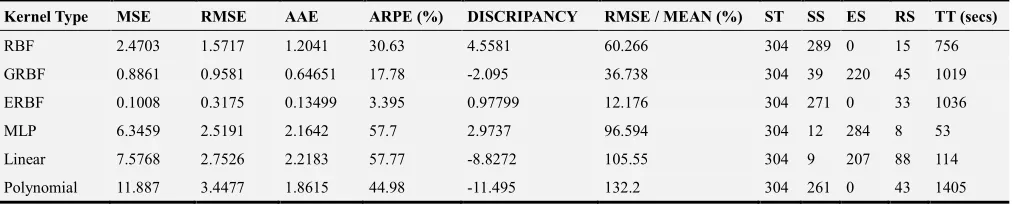
Table 1. SVM Training ratio of 60-20-20 with various kernel functions.
Kernel Type MSE RMSE AAE ARPE (%) DISCRIPANCY RMSE / MEAN (%) ST SS ES RS TT (secs)
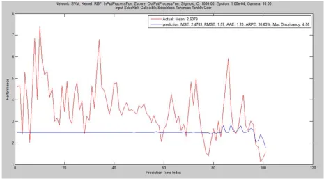
RBF 2.4703 1.5717 1.2041 30.63 4.5581 60.266 304 289 0 15 756
GRBF 0.8861 0.9581 0.64651 17.78 -2.095 36.738 304 39 220 45 1019
ERBF 0.1008 0.3175 0.13499 3.395 0.97799 12.176 304 271 0 33 1036
MLP 6.3459 2.5191 2.1642 57.7 2.9737 96.594 304 12 284 8 53
Linear 7.5768 2.7526 2.2183 57.77 -8.8272 105.55 304 9 207 88 114
Polynomial 11.887 3.4477 1.8615 44.98 -11.495 132.2 304 261 0 43 1405
The result of the first trial with configuration of training ratio 60-20-20 was shown in Table 1 and the corresponding graphical performances of the six different kernels are depicted in Figure 1 to 6. It was deducted that, fair performance was recorded on RBK while ERBK and GRBK outperform MLP, Linear and Polynomial which have performed poorly. The computational time and convergence speeds are relatively high except for that of MLP and linear kernels.
Figure 2. SVM Regression with MLP kernel of training ratio 60-20-20.
Figure 4. SVM Regression with GRBF kernel of training ratio 60-20-20.
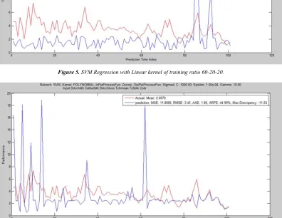
Figure 5. SVM Regression with Linear kernel of training ratio 60-20-20.
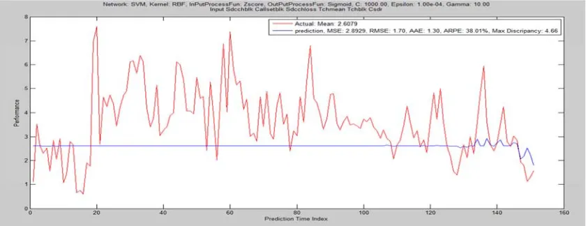
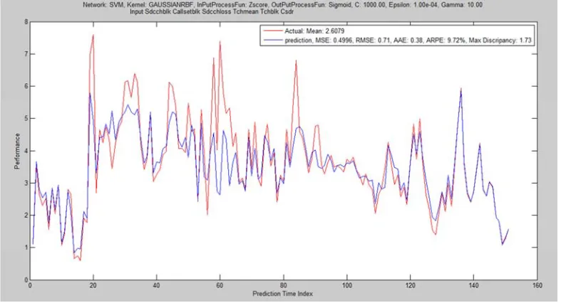
6.2. Training Ratio 40-30-30
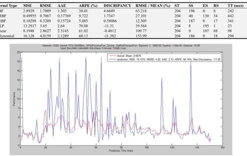
The result of the second trial with configuration of training ratio 40-30-30 was shown in Table 2 and the corresponding graphical performances of the six different kernels are depicted in Figure 7 to 12. It was deducted that, fair performance was recorded on RBK while ERBK and GRBK outperform MLP, Linear and Polynomial which had performed poorly. The computational time and convergence speeds are moderately low except for that of MLP and linear kernels where they were quicker and faster.
Table 2. Training ratio of 40-30-30 with various kernel functions.
Figure 7. SVM Regression with Polynomial kernel of training ratio 40-30-30.
Figure 8. SVM Regression with Linear kernel of training ratio 40-30-30.
Kernel Type MSE RMSE AAE ARPE (%) DISCRIPANCY RMSE / MEAN (%) ST SS ES RS TT (secs)
RBF 2.8929 1.7009 1.303 38.01 4.6649 65.218 204 196 0 8 242
GRBF 0.49955 0.7067 0.37769 9.722 1.7347 27.101 204 40 130 34 442
ERBF 0.10298 0.3209 0.15724 5.085 0.58086 12.305 204 187 0 17 341
MLP 13.2917 3.65 2.64 70.88 -11.31 39.564 204 8 195 1 23
Linear 8.1948 2.8627 2.3143 61.02 -8.4812 109.77 204 9 107 88 98
Figure 9. SVM Regression with RBF kernel of training ratio 40-30-30.
Figure 10. SVM Regression with MLP kernel of training ratio 40-30-30.
Figure 12. SVM Regression with GRBF kernel of training ratio 40-30-30.
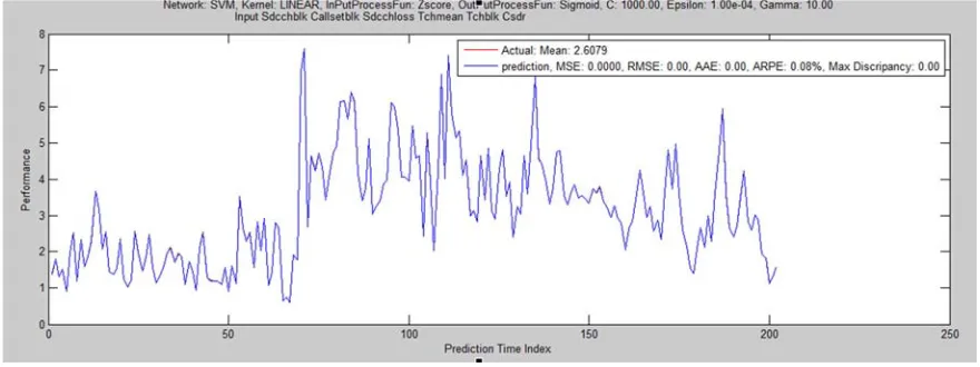
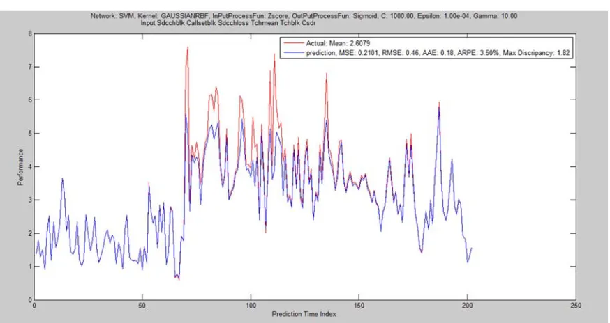
6.3. Training Ratio 20-40-40
The result of the third trial with configuration of training ratio 20-40-40 was shown in Table 3 and the corresponding graphical performances of the six different kernels are depicted in Figure 13 to 18. It was deducted that, fair and best performance was recorded on RBK and Linear kernel respectively while ERBK and GRBK outperform MLP and Polynomial which have performed poorly. The computational time and convergence speeds are very high and encouraging
Table 3. Training ratio of 20-40-40 with various kernel functions.
Kernel Type MSE RMSE AAE ARPE (%) DISCRIPANCY RMSE / MEAN (%) ST SS ES RS TT (secs)
RBF 2.6735 1.6351 1.2277 40.36 5.0313 62.696 102 98 0 4 45
GRBF 0.21006 0.4583 0.17645 3.504 1.8241 17.574 102 32 52 18 72
ERBF 0.16742 0.4091 0.22215 6.824 1.7081 15.689 102 96 0 6 52
MLP 9.4182 3.0689 2.2488 80.31 -9.0588 117.68 102 7 93 2 3
Linear 3.84e-06 0.0019 0.00196 0.082 0.00196 0.07523 102 31 0 71 3
Polynomial 5.7055 2.3886 1.3428 40.33 -9.6637 91.59 102 91 0 11 60
Figure 14. SVM Regression with Linear kernel of training ratio 20-40-40.
Figure 15. SVM Regression with Polynomial kernel of training ratio 20-40-40.
Figure 17. SVM Regression with ERBF kernel of training ratio 20-40-40.
Figure 18. SVM Regression with GRBF kernel of training ratio 20-40-40.
In general, the findings brought about practical recommendations for setting SVM regression parameters which were implemented and underscore the importance of selecting appropriate value of − ! " zone parameter on the generalization performance. It is worth noting that SVM generalization performance (estimation accuracy) depends wholly on a good setting of meta-parameters. The constant 4 that determines the trade-off between the model complexity (flatness) and the degree to which deviations larger than Epsilon ( ) are tolerated in optimization formulation. As the comparisons were made between the different kernel functions for the varied kernel training ratio and fixed kernel parameters, it is deduced that ERBF and GRBF give best classification with good specificity and sensitivity values.
7. Conclusions
Therefore, despite SVMs being limited to making binary classifications, their superior properties of scalability and generalization capability give them an advantage in other domains.
References
[1] Babu, R, Gowrishankar, H. S and Satyanarayana, P, “An Analytical framework for Call Admission Control in Heterogeneous Wireless Networks”, IJCSNS International Journal of 162 Computer Science and Network Security, VOL.9 No.10, October 2009, pp.162-166.
[2] Bordes, A., Bottou, L., and Gallinari, P. Sgd-qn: Careful quasi-newton stochastic gradient descent. JMLR, 2009. [3] Deshmukh, S. B and Deshmukh, V, V (2013), Call Admission
Control in Cellular Network, International Journal of Advanced Research in Electrical, Electronics and Instrumentation Engineering, Vol. 2, Issue 4, April 2013, ISSN (Print): 2320 – 3765, ISSN (Online): 2278 – 8875. [4] Haykin, S. (2009). Neural networks and learning machines.
3rd ed. New Jersey: Pearson Education Inc.
[5] Hoang N. D, Tien Bui D, Liao KW. 2016. Groutability estimation of grouting processes with cement grouts using differential flower pollination optimized support vector machine. Appl Soft Comput. 45:173–186.
[6] Kaitao L, Natalie T, and Aidan, O. (2018). Artificial Intelligence and Machine Learning in Bioinformatics. Encyclopedia of Bioinformatics and Computational Biology doi:10.1016/B978-0-12-809633-8.20325-7.
[7] Kotsiantis, S, Kanellopoulos, D and P. Pintelas, Data Preprocessing for Supervised Leaning. International Journal of Computer Science, Vol. 1, Issue No. 2, 2006; p. 111-117. [8] Kumar, S., Kumar, K and Kumar, P. (2014), A Comparative
Study of Call Admission Control in Mobile Multimedia Networks using Soft Computing, International Journal of Computer Applications (0975 – 8887), Volume 107 – No. 16, December 2014.
[9] Lin, S. W; Lee, Z. J; Chen, S. C. and Tseng, T. Y. “Parameter determination of support vector machine and feature selection using simulated annealing approach,” Applied Soft Computing Journal, vol. 8, no. 4, pp. 1505–1512, 2008.
[10] Muthu R. K, Shuvo Banerjee, Chinmay Chakraborty, Chandan Chakraborty, Ajoy K. Ray, “Statistical analysis of mammographic features and its classification using support vector machine”, Expert Systems with Applications 37, page: 470-478, 2010.
[11] Omolaye P. O., (2014): Management Information Systems Demystified for Managers and Professionals; Selfers Publishers Ltd., Makurdi, Nigeria. ISBN: 978-978-52663-75. [12] Omolaye, P. O., Mom, J. M. and Igwue, G. A (2017). A
Holistic Review of Soft Computing Techniques. Applied and Computational Mathematics; 6(2): 93-110. http://www.sciencepublishinggroup.com/j/acm. doi: 10.11648/j.acm.20170602.15. ISSN: 2328-5605 (Print); ISSN: 2328-5613 (Online).
[13] Qiujun H, Jingli M and Yong L. (2012). An Improved Grid Search Algorithm of SVR Parameters Optimization. Inst. of Elect and Elect Engineering (IEEE). 978-1-4673-2101-3/12. [14] Shanthini, D., Shanthi, M. and Bhuvaneswari, M. C. (2015). A
Comparative Study of SVM Kernel Functions Based on Polynomial Coefficients and V-Transform Coefficients. International Journal of Engineering and Computer Science ISSN:2319-7242 Volume 6 Issue 3 March 2017, Page No. 20765-20769 Index Copernicus value (2015): 58.10 DOI:10.18535/ijecs/v6i3.65.
[15] Singh R. K. and A. Ashtana (2012), “Architecture of wireless network,” International Journal of Soft Computing and Engineering, ISSN: 2231-2307, Volume-2, Issue-1.
[16] Wu, C. F., Lee, L. T., Chang, H. Y. and Tao, D. F (2011), “A novel call admission control policy using mobility prediction and throttle mechanism for supporting QoS in wireless cellular networks,” Journal of Control Science and Engineering, Volume 2011, Article ID 190643, Hindawi Publishing Corporation, doi:10.1155/2011/190643.
[17] Xin W, Arunita J and Ataul Bari (2011a), Optimal Channel Allocation with Dynamic Power Control in Cellular Networks, International Journal of Computer Networks & Communications (IJCNC) Vol.3, No.2, March 2011 DOI: 10.5121/ijcnc.2011.3206 83.
[18] Yukai Y, Hongmei Cui, Yang Liu, Longjie Li, Long Zhang, and Xiaoyun Chen (2015). PMSVM: An Optimized Support Vector Machine Classification Algorithm Based on PCA and Multilevel Grid Search Methods. Hindawi Publishing Corporation, Mathematical Problems in Engineering, Volume 2015, Article ID 320186.
[19] Zhi-ming W, Xian-sheng T, Zhe-ming Y, and Chao-hua W, “Parameters Optimization of SVM Based on Self-calling SVR,” Journal of System Simulation, 2010. 2, vol. 22 No. 2. [20] Chang Y, Hsieh C, Chang K. W, Ringgaard M and Lin C
(2010). Training and testing low-degree polynomial data mappings via linear SVM. Journal of Machine Learning Research. 11:1471-1490.