Effect of Unmodelled Actuator Dynamics on Feedback Linearised
Systems and a Two Stage Feedback Linearisation Method
Mohamed Kara Mohamed and Alexander Lanzon
Abstract— This paper is concerned with the control design of nonlinear systems using feedback linearisation. The paper highlights the destabilisation effect of unmodelled actuator dynamics when applying feedback linearisation. To overcome this difficulty, a two stage feedback linearisation technique is proposed to compensate for actuator dynamics and subse-quently linearise nonlinear systems. A case study of a tri-rotor UAV is used to showcase the benefits of the proposed method in comparison with classical feedback linearisation. The paper is written from a UAV application’s point of view, however, the proposed procedure is still valid for any input-affine invertible nonlinear system.
I. INTRODUCTION
One of the common control design techniques for non-linear systems is to non-linearise the system by cancelling the nonlinearity and then a linear control method can be used to synthesize a controller for the linearised model [5]. Cancelling the nonlinear term via feedback is known as feed-back linearisation, and it can be either state-input feedfeed-back linearisation or input-output feedback linearisation. In this paper, we consider input-output feedback linearisation.
To simplify the implementation of feedback linearisation, several assumptions relating to the model of the nonlinear system and its operating point are considered. One of these assumptions, which is widely accepted in literature, is to neglect actuators dynamics. For instance, actuators dynamics are commonly neglected in Unmanned Aerial Vehicle (UAV) applications when synthesizing a controller (see for example [3], [2], [6] and the references therein). In these references, it is assumed that the actuators are fast and their dynamics can be safely neglected. In this work, we show that this assumption is not always valid and that when it comes to feedback linearisation, unmodeled actuators dynamics can have a vital destabilisation effect.
The effect of actuators dynamics on feedback linearisation has been considered by several research works, see for example [12], [1] and there references therein. However, the focus in these references is on how to recover the stability of the system when actuators dynamics are not available. In this work, we assume that actuators dynamics can be modelled and a two stage feedback linearisation method is then developed to handle actuators dynamics and linearise the nonlinear system. Although [4] tackles a similar problem, the work there is restricted to compensation of
Authors are with the Control Systems Centre, School of Electrical and Electronic Engineering, The University of Manchester, Manchester, UK,
M13 9PL. [email protected],
actuators dynamics only for a specific SISO system. No such restrictions are made here.
The rest of the paper is organized as follows. In Section II, the input-output feedback linearisation technique is briefly reviewed. The undesirable effect of unmodelled actuators dynamics on input-output feedback linearisation is discussed in Section III. In Section IV, a two stage input-output feed-back linearisation algorithm is proposed for a fully modelled system that includes actuators dynamics. A case study of a tri-rotor UAV is investigated in Section V and the summary of the paper is presented in Section VI.
II. INPUTOUTPUTFEEDBACKLINEARIZATION
This section reviews the concept of input-output feedback linearisation [9] used to transform a nonlinear system into a linear one for a subsequent linear control design.
Consider a class of continuous multi-input multi-output (MIMO) fully actuated nonlinear systems of ordernand size
m×mgiven by:
˙
x=f(x) +GGG(x)u (1)
y=h(x) (2)
Satisfying well known conditions, the nonlinear system (1) - (2) can be transformed into a linearised system of global normal form defined in a domainD⊂Rnand given by:
˙
ζ =AAAcζ+BBBcϑ (3)
y=CCCcζ (4)
where Ac, Bc and Cc are block diagonal matrices of the Brunovsky canonical form. ζ =
ζ1 ζ2 · · · ζm
T
is de-fined by a new transformation mapping ζ=T(x) such that each elementζiis a vector of the outputyiand its derivatives up toy(ri−1)
i whereri is the relative degree of the outputyi. The feedback linearisation law from system (1) - (2) to the linearised system (3) - (4) is given by [9]:
u(x,ϑ) =α(x) +βββ(x)−1ϑ, (5)
The matrix βββ(x) is called the decoupling matrix and it is assumed that this matrix is invertible in the domainD. The new artificial input vector is defined as:
ϑ =y(r1)
1 y
(r2)
2 · · · y
(rm) m
T
III. UNMODELLEDACTUATORSDYNAMICS
When applying feedback linearisation, actuators dynamics are usually neglected based on the assumption that actuators are fast enough to apply the required controller action without any considerable delay. In this section, we analyse the effect of unmodeled actuators dynamics on input-output feedback linearisation.
Consider a nonlinear system represented by (1) - (2) with actuators dynamics of ordernarepresented by:
˙
xa=AAAaxa+BBBaua (6)
ya=CCCaxa (7)
We assume that the actuators system is asymptotically stable for all values xa(t)∈D. To impose actuators dynamics on the linearised system, we assume that the mappingζ=T(x) is invertible. Rearranging the artificial control inputϑ to be in terms of the physical input u, the linearised system can be rewritten in terms of the physical input as:
˙
ζ =AAAcζ+BBBcβββ(T−1(ζ))(u−α(T−1(ζ))) (8)
y=CCCcζ (9)
The physical input to the system is now the output of the actuators u=ya=CCCaxa and the feedback linearisation law is feeding to the actuators system ua=α(T−1(ζ)) + β
ββ−1(T−1(ζ))ϑ and therefore the system from ϑ to y per-turbed by actuators dynamics can be represented by:
˙
ζ=AAAcζ+BBBcβββ(T−1(ζ))CCCaxa−BBBcβββ(T−1(ζ))α(T−1(ζ)) (10) ˙
xa=AAAaxa+BBBaα(T−1(ζ)) +BBBaβββ−1(T−1(ζ))ϑ (11)
y=CCCcζ (12)
The perturbed system in (10) - (12) is nonlinear and different from the linearised system (1) - (2). The order of this system fromϑ toyisn+na. There is no guarantee that the synthesized controller for the linearised system in (3) - (4) will be able to stabilize the nonlinear system of higher order in (10) - (11). Moreover, if the controller manages to stabi-lize the nonlinear system, the performance will deteriorate. Therefore, actuators dynamics cannot be always neglected safely when using feedback linearisation as there is risk of instability.
IV. TWOSTAGEFEEDBACKLINEARISATION
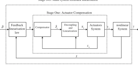
In this section, a two stage feedback linearisation tech-nique is proposed to compensate for actuators dynamics and retain the validity of feedback linearisation of the nonlinear system. In this two stage method, the first stage handles actu-ators dynamics using inner loop linearisation/compensation and the second stage designs the outer loop by linearising the main nonlinear system. Figure 1 represents a block diagram of the proposed two stage feedback linearisation for nonlinear systems with actuators dynamics.
Consider a fully actuated nonlinear MIMO system given by (1) - (2) with actuators dynamics given by a nonlinear MIMO model of similar structure. The complete nonlinear
Actuators System
nonlinear System
a - Decoupling
and Linearization
Feedback linearisation
law
Compensator ua
u
a
x
x
a
y y
Stage One: Actuator Compensation
-Stage two: Main system feedback linearisation
Fig. 1. Block diagram of the proposed two stage feedback linearisation.
system including actuators dynamics from ua to y can be represented by:
˙
x=f(x) +GGG(x)ha(xa) (13)
˙
xa= fa(xa) +GGGa(xa)ua (14)
y=h(x). (15)
With the assumption that the actuators model satisfies the feedback linearisation conditions, the nonlinear actuators system can be linearised using input-output feedback lin-earisation to get:
˙
ζa=AAAaζa+BBBaϑa (16)
ya=CCCaζa, (17)
where AAAa, BBBa, CCCa and ϑa are defined with respect to the actuators system. ζa=
ζa1 ζa2 · · · ζam
is a new actuators state vector defined by the mapping ζa=Ta(xa) such that each elementζai is a vector of the outputyai and its derivatives up toy(riai−1)whererai is the relative degree of the outputyai. System (16) - (17) is a MIMO decoupled system in which each channel can be handled individually. For the i-th SISO channel of the linearised actuators system, let ξi=ζai withξi=
ξi1 ξi2 · · · ξirai
T
, then the dynamics of the i-th linearised channel can be written as:
˙
ξi1 =ξi2 (18)
˙
ξi2 =ξi3 (19)
..
. (20)
˙
ξirai =ϑai (21)
yai=ξi1. (22)
structure as following:
ei1=ξi1−ui (23)
ei2=ξi2−zi1−u˙i (24)
..
. (25)
eirai =ξirai−zi(rai−1)−u
(rai−1)
i , (26)
wherezik, 1≤k≤rai is a backstepping control law that is used to achieve stability and convergence of the overall error system [10]. Using Lyapunov functions,zik can be designed as [10]:
zik=−eik−1−cikeik+z˙ik−1 (27)
The final control law for the i-th channel can be represented as:
ϑai=zirai +u (rai)
i , (28)
The resulting error system from (23) - (26) is given as:
˙
ei1
˙
ei2
.. . ˙
eirai
=
−ci1 1 0 · · · 0
−1 −ci2 1 · · · 0
0 −1 . .. ... ... 0 0 · · · −1 −cirai
ei1
˙
ei2
.. .
eirai
(29)
Using Lyapunov theory, it can be easily proved that the above system in (29) is globally uniformly asymptotically stable at the origin, which means that the global asymptotic tracking is achieved. The transient performance of the error system can be controlled by the design parameters cik. In general, increasing cik will improve the transient performance of the error system [10]. This backstepping control design needs to be repeated for all actuators channels.
Upon completing the control design of the inner loop, one can put now ya≈u assuming a high value of cik to achieve high bandwidth. Thereafter, the second stage can be implemented, which is input-output feedback linearisation of the main nonlinear system only bypassing the inner loop.
One point that might arise here is why the two stage feedback linearisation is needed given that the actuators dynamics are available and the whole system including actua-tors can be linearised in one step using the standard feedback linearisation procedure? The proposed two stage algorithm simplifies the implementation of feedback linearisation and is less conservative for the feedback linearisation law. For instance, consider a full nonlinear system including actuators dynamics as represented by (13) - (15). This system can be linearised as one system using standard feedback lin-earisation. However, this requires differentiation along both vector statesxaandx, which means that the vector functions
f(·), fa(·)and the column functions ofG(·)andGa(·)need to be smooth and differentiable up to the n+na degree. This condition is more conservative and is not required in the two stage feedback linearisation as the actuators system and the plant are handled separately. A comparison study between the proposed two stage feedback linearisation and the standard linearisation on the whole system will be conducted when considering the example of the tri-rotor UAV in next section.
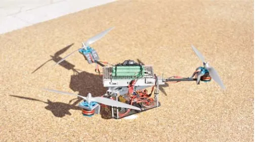
Fig. 2. The tri-rotor UAV system.
V. CASESTUDY: DESIGN ANDCONTROL OFA
TRI-ROTORUAV
This section is dedicated to the control design of a tri-rotor UAV as a case study of using the proposed two stage feedback linearisation to linearise a nonlinear system. The vehicle under consideration was proposed originally in [8] and is shown in Figure 2. The vehicle’s dynamics expressed in the body coordinate system can be described by [8]:
˙
υ=gHg−SSS(ω)υ+
kf
Mtot
H
HHfρ (30)
˙
ω=−(III)−1SSS(ω)IIIω+ (III)−1(k
fHHHt−ktHHHf)ρ (31) ˙
η=ΨΨΨω (32)
˙
λ=RRRebυ (33)
Full definition of the notation and derivation of the model can be accessed in [7]. The output of the system is defined as the position and attitude of the vehicle, i.e.,y=
η λT
. In [8], an H∞ controller was designed to stabilise the
vehicle where input-output feedback linearisation is used to linearised the system. Actuators dynamics were neglected with the assumption that actuators are fast enough to apply the control action without any considerable delay. In this paper, this assumption is analysed and challenged, and then feedback linearisation for the full model that includes actu-ators dynamics is implemented. For convenience and com-parative purposes, the controller designed in [8] is presented here again.
The case study includes 4 scenarios depending on the level of the UAV model and the implemented feedback linearisation as following:
Case 1: The system model does not include actuators dy-namics, which is a replica of the case considered originally in [8].
Case 2: Actuators dynamics are included in the system model but not accounted for by the controller.
Case 3: The proposed two stage feedback linearisation is invoked to linearise the full system, i.e., including actuators dynamics.
Cases 1 and 2 aim to demonstrate the undesirable effect of unmodelled actuators dynamics on feedback linearisation, while Cases 3 and 4 present a comparative study between the proposed two stage feedback linearisation and the classical feedback linearisation on the whole system. The performance of the controller in all cases is simulated using Matlab Simulink software. All simulations are considered for a scenario of horizontal hovering at height of 5 m, i.e., the reference input is(0,0,0)deg for the attitude and (0,0,5)
mfor the position in the earth frame, and the vehicle was at a non-zero initial position and attitude.
1) Case 1: Control Synthesis without Actuators Dynam-ics: As mentioned earlier, this case represents the controller synthesised in [8] where no actuators dynamics are consid-ered. In this case, the vectorρin (30) is considered as the the input vector of the system, i.e., u=ρ. The linearised plant is a double integrator representing single degree of freedom for translational and rotational motion and the feedback linearisation law is derived as:
u=βββ−1
ϑ−
˙
Ψ
ΨΨ−ΨΨΨIII−1SSS(ω)III
ω
gRRRebHg
. (34)
whereϑ byy(2)=ϑ and the matrix βββ is defined as:
β β β =
ΨΨΨIII−1kfHt−ktHHHf
kf MtotRRR
e bHHHf
. (35)
It has been shown thatdet[βββ(.)]= 0 and the inverseβββ(.)−1
always exists for all states values of the system. Using the synthesisedH∞LSDP controller in [8], the vehicle’s position
(xv,yv,zv) and attitude (pitchφv, rollθv, yaw ψv) related to the earth coordinate system and the control efforts in terms of the BLDC motors speeds ωmi and the tilting angles of the servo motors αsi are shown in Figures 3(a) and 3(b) respectively.
2) Case 2: Analysis of The Effect of Unmodeled Actuators
Dynamics: In the previous case, actuators dynamics were
neglected assuming that actuators are fast and their dynamics can be neglected. In this case, we challenge this assumption by investigating the effects of unmodeled actuators dynamics on the stability of the system.
The tri-rotor UAV has two types of actuators, BLDC motors and digital Servos. Neglecting the inductance effect, the dynamic model of the BLDC motors can be represented by a first order system [11]. Similarly, the servos combined with their drive circuits can be represented by first order systems using the supplied specifications of the servos step responses. Assuming identical BLDC motors and identical servo motors, and in state space form, the dynamics of the six actuators (three BLDC motors and three servo motors) can be written as:
˙
xa=AAAaxa+BBBaua (36)
ya=xa (37)
whereAAAaandBBBaare diagonal matrices with suitable dimen-sion. ya is a vector of the rotational speeds of the BLDC
0 2 4 6 8 10 í0.2
0 0.2 0.4 0.6
xv
(m)
time (s)
0 2 4 6 8 10 í3
í2 í1 0 1
yv
(m)
time (s)
0 2 4 6 8 10 2
3 4 5 6
zv
(m)
time (s)
0 2 4 6 8 10 0
2 4 6
φv
(deg)
time (s)
0 2 4 6 8 10 í20
í10 0 10
θv
(deg)
time (s)
0 2 4 6 8 10 í5
0 5 10 15
ψv
(deg)
time (s)
(a) The UAV position and attitude.
0 1 2 3 4 5 6 7 8 9 10 í100
í50 0 50 100
Servo Angles (Deg)
time (s)
αs1
αs2
αs
3
0 1 2 3 4 5 6 7 8 9 10 2000
4000 6000 8000 10000 12000
Motors speed (RPM)
time (s)
ωm
1
ωm
2
ωm
3
(b) The actuators performance.
Fig. 3. Case1: Control design for system without actuators dynamics [8].
motors and angles of the servo motors. ua is the driving voltages of the BDLC motors and the servo motors.
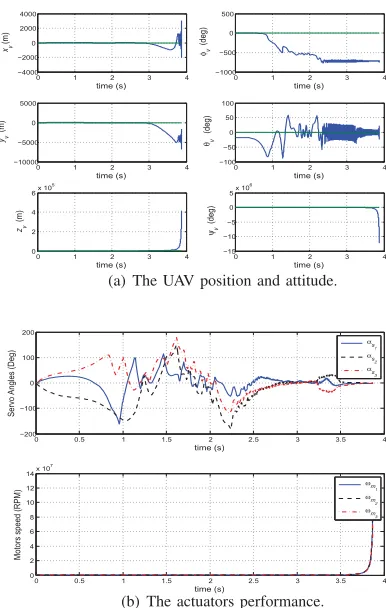
We now include the actuators dynamics in the simulation using the same controller considered in Case 1 to test the stability of the system. The effect of the unmodelled actuators dynamics on the performance of the UAV is reflected in Figure 4(a) with actuators effort shown in Figure 4(b). These figures clearly show that unmodelled actuators dynamics destabilize the UAV system. This observation is consistent with the result derived before in Section III.
3) Case 3: Two Stage Feedback Linearisation Technique:
In this case, we invoke the two stage feedback linearisation technique developed in Section IV to linearise the system and then design an H∞ controller. As the actuators system is a
linear decoupled system, there is no need for a linearisation or decoupling process and the backstepping technique can be applied directly. The error system is defined as:
e=ya−yd, (38)
whereyd=u anduis the feedback linearisation law of the outer loop (to be designed later). This means:
˙
e=y˙a−y˙d (39)
=AAAaxa+BBBaua−y˙d (40)
We nominate the Lyapunov functionV=1
2e
2, whose
0 1 2 3 4 í4000 í2000 0 2000 4000 xv (m) time (s)
0 1 2 3 4 í10000 í5000 0 5000 yv (m) time (s)
0 1 2 3 4 0
2 4 6x 10
5
zv
(m)
time (s)
0 1 2 3 4 í1000 í500 0 500 φv (deg) time (s)
0 1 2 3 4 í100 í50 0 50 100 θv (deg) time (s)
0 1 2 3 4 í15
í10 í5 0 5x 10
6
ψv
(deg)
time (s)
(a) The UAV position and attitude.
0 0.5 1 1.5 2 2.5 3 3.5 4 í200
í100 0 100 200
Servo Angles (Deg)
time (s) α s1 α s2 α s3
0 0.5 1 1.5 2 2.5 3 3.5 4 0 2 4 6 8 10 12 14x 10
7
Motors speed (RPM)
time (s) ω m1 ω m2 ω m3
(b) The actuators performance.
Fig. 4. Case2: The undesirable destabilizing effect of unmodelled actuators dynamics.
stability at the origin, we design the control law, following Eq. (28), as:
ua=BBB−a1[y˙d−AAAaxa−ccce] (41)
=BBB−a1[u˙−AAAaxa−ccc(xa−u)] (42)
whereccc is a diagonal design matrix. To ensure high band-width and quick convergence of ya toyd, we chooseccc with large elements. Typically, cii>100,i=1,2· · ·,6, where cii are the diagonal elements of the matrixccc, are sufficient.
We now move to the second stage where we linearise the UAV system without the inner loop. This stage includes the linearisation of the UAV system as described in (30) -(33). The feedback linearisation law is given in (34) and the resulting linearised system is a double integrator.
To demonstrate the system performance when using the two stage feedback linearisation, we implement the same controllers designed before in Case 1. In Figures 5(a) and 5(b) respectively, the system performance and the actuators efforts are depicted. It can be noted that Figure 5 is very similar to Figure 3 where actuators dynamics were not included. This is due to the inner stage of compensating and controlling actuators dynamics.
4) Case 4: Complete Model Classical Feedback
Lineari-sation: For comparative study, classical feedback
linearisa-tion of the full system including actuators dynamics is im-plemented in this case. The study aims to clarify the benefits
0 2 4 6 8 10 í0.2 0 0.2 0.4 0.6 xv (m) time (s)
0 2 4 6 8 10 í4 í2 0 2 yv (m) time (s)
0 2 4 6 8 10 0 2 4 6 zv (m) time (s)
0 2 4 6 8 10 0 2 4 6 φv (deg) time (s)
0 2 4 6 8 10 í20 í10 0 10 θv (deg) time (s)
0 2 4 6 8 10 í5 0 5 10 15 ψv (deg) time (s)
(a) The UAV position and attidute.
0 1 2 3 4 5 6 7 8 9 10 í100
í50 0 50 100
Servo Angles (Deg)
time (s)
αs
1
αs
2
αs3
0 1 2 3 4 5 6 7 8 9 10 0 2000 4000 6000 8000 10000 12000
Motors speed (RPM)
time (s) ωm 1 ωm 2 ωm 3
(b) The actuators performance.
Fig. 5. Case3: Control design for the full system using the two stage
feedback linearisation associated withH∞LSDP.
of the proposed two stage feedback linearisation technique. The complete model of the tri-rotor UAV including actuators dynamics is:
˙
υ=gHg−SSS(ω)υ+
kf
Mtot
H
HHfρ (43)
˙
ω=−III−1SSS(ω)IIIω+III−1(kfHHHt−ktHHHf)ρ (44) ˙
η=ΨΨΨω (45)
˙
λ=RRRebυ (46)
˙
xa=AAAaxa+BBBaua (47)
ya=xa. (48)
The input to the system is ua and implementing input-output feedback linearisation gives the following feedback linearisation law:
ua=βββ−f1
ϑf−CCC111ρ−C2
, (49)
where
C C C111=
2 ˙ΨΨΨIII−1−ΨΨΨIII−1SSS(ω) +ΨΨΨIII−1SSS(IIIω)III−1 kfHHHt−ktHHHf kf
MtotRRR
e bSSS(ω)HHHf
,
(50)
C2= ¨
ΨΨΨ−2 ˙ΨΨΨIII−1SSS(ω)III−ΨΨΨIII−1SSS(IIIω)III−1SSS(ω)III ω
gRRRebSSS(ω)Hg
+
Ψ Ψ
ΨIII−1SSS(ω)SSS(ω)III ω
gRRRebHHHdgΨΨΨω
+
Ψ ΨΨIII−1
kfHHHt−ktHHHf
kf
MtotRRR
e bHHHf
N N NAAAaxa,
and
NNN=
diag(2ωmisinαsi) diag(ω
2
micosαsi)
diag(2ωmicosαsi) diag(−ω
2
misinαsi)
6×6
,i=1,2,3
(52)
HHHdg=
cos(θv) 0 0
sin(θv)sin(θv) −cos(φv)cos(θv) 0
cos(θv)sin(θv) sin(φv)cos(θv) 0
. (53)
The decoupling matrix is defined as:
β β βf=
Ψ
ΨΨIII−1kfHHHt−ktHHHf
kf
MtotRRR
e bHHHf
N N
NBBBa. (54)
and its determinant is det[βββf(.)] =−kdωm31ω
3
m2ω
3
m3/cos(θv)
wherekd is a positive constant related to the specifications of the vehicle. This means that βββf(.) is invertible and the feedback linearisation law exists as long as the BLDC motors are operating and the cos(θv)=0 . Therefore, the motors should be switched on and operate at low speeds before the controller takes an action to avoid any mathematical error during the initial start of the vehicle. The new control input ϑf is defined as ϑf =y(3) and the linearised system is a chain of triple integrators with no internal dynamics. The
H∞ LSDP is now invoked to synthesize a controller for
the full linearised system using the standard weight design specification of high gain at low frequency and low gain at high frequency in addition to reasonable bandwidth.
Performance of the UAV system and the actuators efforts of this case are shown in Figures 6(a) and 6(b) respectively. Comparing the decoupling matrices and the feedback linearisation law in both cases, Case 3 (as in (34)) and Case 4 (as in (49)), highlights the strengths of the proposed two stage feedback linearisation technique. The feedback linearisation law resulting from the proposed method is exists for all values of the system states due to the fact that the decoupling matrixβββ in (35) is always nonsingular. In contrary, the decoupling matrix βββf in (54) is singular when any of BLDC motor has zero speed or when the roll angle θv of the vehicle is close to π/2. This means that the controller of the two stage feedback linearisation can work for all positions and attitudes of the vehicle and all speeds and angles of the actuators while the feedback linearisation law in Case 4 does not exist for all state values, i.e. when the BLDC motors are not operating singularity exist, and the controller cannot start from static. In terms of performance and actuators efforts, the reader can notice also that the system reaches the steady state value faster when using the two stage feedback linearisation, and this is due to the compensation and control of actuators dynamics in the inner loop.
VI. SUMMARY
This paper shows the vital importance of actuators dy-namics for the control design of nonlinear systems when using dynamic inversion. To implement input-output feed-back linearisation while considering actuators dynamics, a two stage feedback linearisation method is developed. The proposed method simplifies the implementation of feedback linearisation when actuators dynamics are considered.
0 2 4 6 8 10 í2
í1 0 1
xv
(m)
time (s)
0 2 4 6 8 10 í4
í2 0 2
yv
(m)
time (s)
0 2 4 6 8 10 0
2 4 6 8
zv
(m)
time (s)
0 2 4 6 8 10 0
2 4 6
φv
(deg)
time (s)
0 2 4 6 8 10 í20
í10 0 10
θv
(deg)
time (s)
0 2 4 6 8 10 í5
0 5 10 15
ψv
(deg)
time (s)
(a) The UAV position and attitude.
0 1 2 3 4 5 6 7 8 9 10 í100
í50 0 50 100 X: 0.8066
Y: 71.21
Servo Angles (Deg)
time (s)
X: 0.8066 Y: í72.89
αs
1
αs
2
αs3
0 1 2 3 4 5 6 7 8 9 10 2000
4000 6000 8000 10000 12000 X: 0.1929
Y: 1.095e+004
Motors speed (RPM)
time (s)
ωm
1
ωm
2
ωm
3
(b) The actuators performance.
Fig. 6. Case4: Control design for the full system using classical feedback
linearisation associated withH∞ LSDP.
REFERENCES
[1] R. W. Aldhaheri and H. K. Khalil. Effect of unmodeled actuator
dynamics on output feedback stabilization of nonlinear systems.
Au-tomatica, 32(9):1323–1327, 1996.
[2] G. Cai, B. M. Chen, K. Peng, M. Dong, and T. H. Lee. Modeling and
control of the yaw channel of a UAV helicopter. IEEE Transactions
on Industrial Electronics,, 55(9):3426–3434, 2008.
[3] J. Chen and Y. Wang. The guidance and control of small net-recovery
UAV. InProceedings of The 2011 Seventh International Conference
on Computational Intelligence and Security (CIS), pages 1566 – 1570, Hainan, China, December 2010.
[4] D. Chwa, J. Y. Choi, and J. H. Seo. Compensation of actuator
dynamics in nonlinear missile control.IEEE Transactions on Control
Systems Technology, 12(4):620–626, 2004.
[5] A. Isidori. Nonlinear Control Systems. Communications and Control
Engineering. Springer, 3 edition, 1995.
[6] Y. Kang and J. K. Hedrick. Linear tracking for a fixed-wing UAV using
nonlinear model predictive control. IEEE Transactions on Control
Systems Technology, 17(5):1202–1210, 2009.
[7] M. Kara Mohamed. Control and Design of UAV Systems, A
Tri-rotor UAV Case Study. Phd thesis, School of Electrical and Elctronic Engineering, The Univeristy of Manchester, UK, 2012.
[8] M. Kara Mohamed and A. Lanzon. Design and control of novel
tri-rotor UAV. In Proceedings of The 2012 UKACC International
Conference on Control, pages 304–309, Cardiff, UK, September 2012.
[9] H. A. Khalil.Nonlinear Systems. Prentice Hall, Inc., 2 edition, 2001.
[10] M. Krsti´c, I. Kanellakopoulos, and P. Kokotovi´c. Nonlinear and
Adaptive Control Design. Adaptive and Learning Systems for Signal Processing, Communications, and Control. Wiley-Blackwell, 1995.
[11] B. C. Kuo.Automatic Control Systems. Wiley & Sons Inc., 7 edition,
1995.
[12] M. S. Mahmoud and M. Zribi. Robust output feedback control for
nonlinear systems including actuators. Systems Analysis Modelling
![Fig. 3.Case1: Control design for system without actuators dynamics [8].](https://thumb-us.123doks.com/thumbv2/123dok_us/1022671.1602314/4.612.322.521.52.365/fig-case-control-design-actuators-dynamics.webp)