Investigating Spatial Error Structures in Continuous Raster Data

Contents lists available atScienceDirect

Int J Appl Earth Obs Geoinformation

journal homepage:www.elsevier.com/locate/jag

Investigating spatial error structures in continuous raster data

Narumasa Tsutsumida

, Pedro Rodríguez-Veiga

, Paul Harris

, Heiko Balzter

,

Alexis Comber

a_{Graduate School of Global Environmental Studies, Kyoto University, Kyoto, 606-8501, Japan} b_{Centre for Landscape and Climate Research, University of Leicester, Leicester, LE1 7RH, UK} c_{NERC National Centre for Earth Observation (NCEO), University of Leicester, Leicester, LE1 7RH, UK} d_{Sustainable Agriculture Sciences, Rothamsted Research, North Wyke, Okehampton, EX20 2SB, UK} e_{School of Geography, University of Leeds, Leeds LS2 9JT, UK}

A R T I C L E I N F O

Keywords: Error distribution Spatial accuracy Local error diagnostics Spatial heterogeneity

A B S T R A C T

The objective of this study is to investigate spatial structures of error in the assessment of continuous raster data. The use of conventional diagnostics of error often overlooks the possible spatial variation in error because such diagnostics report only average error or deviation between predicted and reference values. In this respect, this work uses a moving window (kernel) approach to generate geographically weighted (GW) versions of the mean signed deviation, the mean absolute error and the root mean squared error and to quantify their spatial varia-tions. Such approach computes local error diagnostics from data weighted by its distance to the centre of a moving kernel and allows to map spatial surfaces of each type of error. In addition, a GW correlation analysis between predicted and reference values provides an alternative view of local error. These diagnostics are applied to two earth observation case studies. The results reveal important spatial structures of error and unusual clusters of error can be identified through Monte Carlo permutation tests. Thefirst case study demonstrates the use of GW diagnostics to fractional impervious surface area datasets generated by four different models for the Jakarta metropolitan area, Indonesia. The GW diagnostics reveal where the models perform differently and similarly, and found areas of under-prediction in the urban core, with larger errors in peri-urban areas. The second case study uses the GW diagnostics to four remotely sensed aboveground biomass datasets for the Yucatan Peninsula, Mexico. The mapping of GW diagnostics provides a means to compare the accuracy of these four continuous raster datasets locally. The discussion considers the relative nature of diagnostics of error, determining moving window size and issues around the interpretation of different error diagnostic measures. Investigating spatial structures of error hidden in conventional diagnostics of error provides informative de-scriptions of error in continuous raster data.

1. Introduction

All spatial data are subject to error. Remotely sensed (RS) imagery routinely contains sensor-related errors, atmospheric effects, and geo-metric errors. Environmental datasets that describe landscape features and properties from RS products (e.g. forest aboveground biomass, species distribution, and climate change scenarios) inherently contain prediction errors. Errors can manifest themselves as systematic devia-tions and/or noise which require careful assessment in order to avoid mis-interpretations of the data, to support reliable conclusions and to make informed decisions (Daly, 2006;Foody, 2002). Error assessments provide a guide to data quality and reliability (Foody, 2002) and can provide earth observation (EO) scientists with an understanding of the

sources of error both in RS imagery and products (Liu et al., 2007; Stehman and Czaplewski, 1998). However, conventional summary measures of error do not take any spatial information (e.g. spatial heterogeneity) of error into account (Foody, 2005, 2002). Spatially explicit approach for the assessment is hence important.

In EO studies, spatial extensions of conventional diagnostics of error or accuracy have been demonstrated for categorical raster data, such as land cover classification data (Comber et al., 2017, 2012; Comber, 2013;Congalton, 1988;Foody, 2005). These approaches spatially ex-tend the usual method of estimating and reporting accuracy through a confusion matrix, which is the cross-tabulation of predicted and re-ference classes to generate measures of user’s and producer’s accuracy that correspond to commission and omission errors, respectively, along

https://doi.org/10.1016/j.jag.2018.09.020

Received 10 July 2018; Received in revised form 28 September 2018; Accepted 28 September 2018

⁎_{Corresponding author at: Yoshidahonmachi, Sakyo, Kyoto, 606-8501, Japan.}

E-mail address:[email protected](N. Tsutsumida).

Int J Appl  Earth Obs Geoinformation 74 (2019) 259–268

0303-2434/ © 2018 The Authors. Published by Elsevier B.V. This is an open access article under the CC BY-NC-ND license (http://creativecommons.org/licenses/BY-NC-ND/4.0/).

with an overall accuracy (Congalton, 1991;Stehman and Czaplewski, 1998). Specifically, Comber (2013) demonstrated the use of a geo-graphically weighted (GW) approach to generate spatial surfaces of these measures. The GW approach calculates a series of local diag-nostics of accuracy, using data weighted by their distance to the centre of a moving window or kernel to explore spatial heterogeneity (Gollini et al., 2015). This has been used to compare global land cover datasets (Comber et al., 2013), to assess the consistency of such classification over time (Tsutsumida and Comber, 2015), and to construct hybrid global land cover datasets from multiple inputs (See et al., 2015). Comber et al. (2017) proposed GW confusion matrices for further generic applications. The GW framework itself (Fotheringham et al., 2002; Gollini et al., 2015; Lu et al., 2014) has been widely adopted across many scientific disciplines (e.g. Geography, Ecology, Health), where GW regression (Brunsdon et al., 1996) is the most popular GW model.

The developments of spatially explicit approaches for error assess-ment in continuous raster data in the EO domain have been limited. Comber et al. (2012) proposed a fuzzy GW difference analysis which estimates absolute deviations between the predicted and reference fuzzy membership, essentially applying a fuzzy generalization of the categorical accuracy measures.Khatami et al. (2017)proposed a spatial interpolation approach for soft classification maps in which a linear kernel function was applied to interpolate spatial deviations between predicted and reference proportions, with a focus on weight of spectral or class proportion as a soft classification measure. Willmott and Matsuura (2006)described maps of cross-validation error. Continuous raster data are commonly assessed using mean signed deviation (msd), mean absolute error (mae), root mean square error (rmse) and Pear-son’s correlation coefficient (r). Accurate predictions are reflected by msd, mae and rmse to be zero, coupled withrto be one. Although these conventional diagnostics are useful in reporting error, each of them provides an overall, global or‘whole map’measure only. In this respect, Harris and Juggins (2011)demonstrated GWrfor assessing UK fresh-water acidification prediction accuracy. Harris et al. (2013) demon-strated GW mae for UK freshwater acidification and London house price prediction accuracy, as separate case studies. Monteys et al. (2015) demonstrated GWr for assessing water depth prediction accuracy in

Irish coastal waters. These studies either directly extend GW summary statistics (e.g. GW averages, GW variances) as first proposed by Brunsdon et al. (2002), or directly use GW r (Fotheringham et al., 2002), but in a model accuracy context. Further advances of GW summary statistics can be found in Harris and Brunsdon (2010)and Harris et al. (2014). However, the previous studies have only reported spatial error briefly as part of a suite of diagnostics. That is, spatial extensions of conventional diagnostics of error for continuous raster data have not been described in a comprehensive way, specifically in an EO context. Here we demonstrate the linked use of all four diagnostics, msd, mae, rmse andr, through their GW msd, GW mae, GW rmse and GWrcounterparts and advance them through the application of Monte Carlo permutation tests to identify unusual clusters of error applied to two EO case studies. The first case study evaluates datasets of the fractional impervious surface area (%ISA) with the aim of investigating spatial structures of error in multiple predictions by four different models. The second case study evaluate four different forest above-ground biomass (AGB) datasets in order to compare spatial structures of error in multiple independent datasets.

2. Case study data

2.1. Study 1

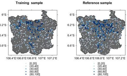
and Comber, 2015). Whenfine resolution images were not available at a sampling grid in 2012, %ISA were interpolated from images dated before and after the year 2012, only if the %ISA is stable over the period (in most cases, %ISA is zero). It is a reasonable approach because im-pervious surfaces do not change frequently. The reference values of % ISA were interpreted twice to minimize human error. The sample grids were randomly divided into training (n= 434) and reference data (n= 550) as shown inFig. 1.

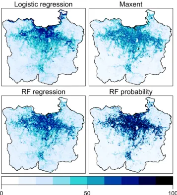
Four different models were implemented to predict %ISA in the JMA: Logistic regression, Maximum Entropy (MaxEnt), Random Forest (RF) regression, and class probability of the RF classifier (hereafter RF probability). All four models return a continuous classification value between 0–100%. Logistic regression is a parametric generalized linear model for response data following a binomial distribution. The out-comes are within the range between 0 and 1 (rescaled to 0–100%). MaxEnt is a non-parametric model, which naturally extends from lo-gistic regression (Phillips and Dudík, 2008). MaxEnt returns the prob-ability of presence from presence-only training data (i.e. without la-belled“absent”data), resulting %ISA predictions. RF regression and RF probability are machine learning techniques using ensemble logistic trees (Breiman, 2001). For RF regression, each tree is constructed by bootstrapped random sampling so that random sample selection leads to a weak correlation between trees. For RF probability, each tree votes for the most popular class and a random sample selection to grow trees

is used to minimize the classification error. Due to its voting system, RF produces a probability of class presence, predicting %ISA. The %ISA predictions of these four models are different and clearly vary spatially (Fig. 2). Note that apparent water surfaces are masked by a MODIS MOD44 W product which represents the water surface in the same spatial scale of the MOD13Q1. Thus, submerged areas (e.g., those found in the North-East edge of the JMA) are excluded in this analysis.

2.2. Study 2

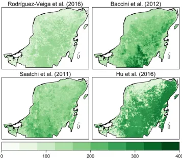
In order to explore how spatial structures of error can differ ac-cording to available different datasets, four AGB spatial datasets for the Campeche, Yucatan, and Quintana Roo administrative regions in the Yucatan peninsula, Mexico are used (Fig. 3). These were developed by Rodríguez-Veiga et al. (2016); Baccini et al. (2012); Saatchi et al. (2011), andHu et al. (2016). Details of these datasets are summarized inTable 1. Dry forest, moist forest, and mangrove forest are found in the North-Western region, the central region, and the coastal zone of the Yucatan peninsula. It is not possible to objectively determine which dataset is the most accurate fromTable 1, as the reported errors are derived from different reference sources. The reference data for this case study was provided by the INFySin-situobservation data which record measures of AGB (Mg ha−1) at four nested 0.04 ha subplots within 1 hafield plots (Rodríguez-Veiga et al., 2016). Data from a total Fig. 2.Predicted fractional impervious surface area (%) by four models for study 1: Logistic regression (Left upper), MaxEnt (Right upper), RF regression (Left bottom), and RF probability (Right bottom).

of 286 (1 ha)field plots were used as reference measures of AGB for the period 2004–2007 (Fig. 4). It is noted that the spatial resolution of assessed AGB datasets and reference sample is different, which is a limitation of data availability, similar to the study ofRodríguez-Veiga et al. (2016).

3. Methods

The GW versions of msd, mae, rmse, andrare described as follows. At any locationi, GW msd:gw msd x y. ( , )i i, GW mae:gw mae x y. ( , )i i , and GW rmse:gw rmse x y. ( , )i i are defined as:

= = −

=

gw msd x y. ( , )i i

Σ ω y x Σ ω

( ) j n _ij

j j

j n _ij 1

1 (1)

= = −

=

gw mae x y. ( , )i i

Σ ω y x Σ ω

| | j

n _ij j j

j n _ij 1

1 (2)

and

= = −

=

gw rmse x y. ( , )i i

Σ ω y x Σ ω

( ) j n _ij

j j

j n _ij

1 2

1 ₍₃₎

wherexj andyj are the reference and predicted values at sample location j, respectively, ωij weights controlled by a distance-decay kernel function (Eq.(8)) with respect to locationi andj, andnis the total number of sample data points. Observe that this always holds, msd ≤mae≤rmse (Willmott and Matsuura, 2005) and their GW counter-parts have the same characteristics.

A GWrat any locationi, is found using:

= gw cor x y. ( , )i i

c x y s x s y

( , ) ( ) ( )

i i

i i (4)

where a GW standard deviation:s x( )i is

= = −

=

s x( )i

Σ ω x m x Σ ω

( ( )) j

n _{ij j i}

j n _ij

1 2

1 ₍₅₎

and a GW mean:m x( )i is

= =

=

m x( )i Σ ω x

Σ ω j n _{ij j}

j n _ij

1

1 ₍₆₎

with a GW covariance:c x y( , )i i

= = − −

=

c x y( , )i i

Σ ω x m x y m y Σ ω

[( ( ))( ( ))] j

n _{ij j i j i}

j n _ij 1

1 (7)

For both case studies, the weightsωijare found using a bi-square kernel as follows:

= ⎧

⎨ ⎩ ⎛ ⎝ −

⎞

⎠ <

( )

ω if d b

otherwise

1 | | ,

0 ij

d

b ij

2 2 ij

(8) wheredijis the Euclidean distance between locationsiand j, and the kernel bandwidthb is specified either as a fixed distance or an adaptive distance which includes afixed number of data points for the local diagnostic calculation. In this study, an adaptive kernel was used as it suits the reference points of both case studies were not distributed uniformly. Its size was arbitrarily defined as 10% of nearby data to locationi. The validity of this subjective bandwidth size is discussed in detail in Section5.

permutation tests. These tests can be adapted for GW error diagnostics (GW msd, GW mae, and GW rmse), in order to identify clusters where the diagnostics are‘significantly’or‘unusually’different to what would be found by chance or because of random variation in the error. Pre-dicted and reference sample pairs are successively randomized (999 times in this study) and the local diagnostics are found after each randomization. A‘significance test’is then possible by comparing actual results with results from a large number of randomized distributions (i.e. by ranking all 1000 outcomes and ascertaining where the single, actual outcome lies). In this instance, the randomization hypothesis is that any pattern seen in the error occurs by chance and therefore any permutation of the error is equally likely. For GWr, the arguments are analogous, but where the investigation centers on the correlation be-tween the predicted and reference values, rather than some summary of the error. In all instances, the permutation test should be viewed as informal and conditional on the GW diagnostic specification (i.e. bandwidth size, kernel type, etc.). Thus, throughout this study, the term ‘significance’is used in an informal manner also, for this test.

In addition to calculating the global diagnostics of msd, mae, rmse andr, estimates andp-values for the significance of the Moran’sIof the deviation between predicted and reference values were calculated. These provide useful context and global information about spatial au-tocorrelation in the error. Weights were generated using an inverse distance squared function for the Moran’sIcalculations.

4. Results

4.1. Study 1

Table 2summarizes the conventional diagnostics of msd, mae, rmse, r and the Moran’s I of %ISA predictions from logistic regression, MaxEnt, RF regression and RF probability. The negative msd values indicate that all four models under-predict, where RF regression pro-vides the closest msd to zero (−2.95) and less errors than the other three models, with the smallest mae (15.51) and rmse (21.34) and the largestr(0.73). The logistic regression is the second most accurate with mae (15.77), rmse (21.87), andr(0.72). RF probability is the poorest predictor of %ISA as it shows the largest mae and rmse together with the smallestr, of all four models. All four models show significant spatial autocorrelations in their errors, where all p-values for the

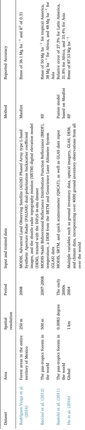
Table 1 Descriptions of four forest aboveground biomass datasets used for study 2. Dataset Area Spatial resolution Period Input and trained data Method Reported Accuracy Rodríguez-Veiga et al. (2016) Forest areas in the entire territory of Mexico 250 m 2008 MODIS, Advanced Land Observing Satellite (ALOS) Phased Array type L-band Synthetic Aperture Radar (PALSAR) dual-polarization backscatter coe ffi cient images, and the shuttle radar topography mission (SRTM) digital elevation model (DEM), trained with the INFyS in-situ dataset MaxEnt Rmse of 36.1 Mg ha − 1and R 2 of 0.31 Baccini et al. (2012) The pan-tropics forests in the world 500 m 2007-2008 MODIS Nadir Bidirectional Re fl ectance Distribution Function Re fl ectance (BRDF), temperature, a DEM from the SRTM and Geoscience Laser Altimeter System (GLAS) data RF Rmse of 50 Mg ha − 1for tropical America, 38 Mg ha − 1 for Africa, and 48 Mg ha − 1for Asia Saatchi et al. (2011) The pan-tropics forests in the world 0.0083 degree The early 2000s MODIS, SRTM, and quick scatterometer (QSCAT), as well as GLAS data input Fusion model based on MaxEnt Relative error of 27.3% for Latin America, 31.8% for Africa, and 33.4% for Asia Hu et al. (2016) Global 1 km 2004 Multiple variables such as ground inventory data, optical imagery, GLAS, DEM, and climate data, incorporating over 4000 ground inventory observations from all over the world RF Rmse of 87.53 Mg ha − 1

Fig. 4.The spatial distribution of in-situ reference sample points for forest aboveground biomass data (units: Mg ha−1) in the Yucatan peninsula, Mexico.

Table 2

Global diagnostics and Moran’sIof fractional impervious surface area predicted by four different models for study 1.

msd mae rmse r Moran’sI* Logistic regression −3.63 15.77 21.87 0.72 0.11

MaxEnt −7.57 15.83 22.74 0.72 0.11

RF regression −2.95 15.51 21.34 0.73 0.06 RF probability −5.12 15.85 24.22 0.71 0.05

* Allp-values for estimates of Moran’sIare less than 0.05.

Moran’sIestimates were less than 0.05. Nevertheless, no local spatial information about the errors is reported inTable 2.

Next, the spatial structure of the errors resulting from the %ISA predictions were explored using the three GW error diagnostics, to-gether with GWrbetween the predicted and reference values as shown inFig. 5. Maps of GW msd indicate where the %ISA values are over- or under-predicted, with positive values representing over-prediction. The GW mae and rmse maps reflect the magnitude of errors (absolute and root squared deviation, respectively, see also Section5). GWrdepicts how the specified correlation varies across the JMA. Results for the associated Monte Carlo permutation tests are highlighted forp-values less than 0.01.

The GW msd results generally suggest that %ISA predictions are under-predicted when compared to reference values, especially in the urban core. Permutation tests locate ‘significant’ areas of unusually large, positive and negative GW msd values. A cluster of‘significantly’ under-predicted values can be found in the middle of the JMA from all four models.

The GW mae and GW rmse maps show that peri-urban areas (sur-rounding the city core) tend to have larger mae/rmse values than others, suggesting the difficulty in predicting %ISA in complex urban frontiers between urban/non-urban areas. ‘Significant’ local clusters differ according to the models, but they tend to be distributed along such urban frontiers.

The results for GWrshow South-Western and South-Eastern areas have consistently weak negative correlations in all four models, and the permutation tests indicate that such correlations are ‘significantly’ unusual for all models. As GWrrepresents spatial variation in the slope of the linear relationship between the predicted and reference values, maps of GWrcan behave differently from those of the other three GW diagnostics which relate to error. Here only the GW mae and GW rmse maps show similarities to each other as expected (see Section 5). As would also be expected from the results ofTable 2, RF regression tends to provide the best local accuracy in most areas, but with clear spatial variation in this accuracy.

4.2. Study 2

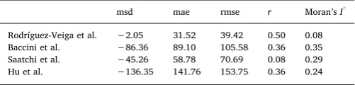
Conventional diagnostics for the four AGB datasets are shown in Table 3. Rodríguez-Veiga’s dataset clearly provides the best accuracy amongst the four AGB datasets, as is evident from the closeness to zero of msd (−2.05), the smallest mae (31.52), the smallest rmse (39.42), and the largestr(0.50). Hu’s dataset is clearly the least accurate. The Moran’sIestimates are all significant (p-values were less than 0.05), indicating the possibility of existing a spatial structure to the errors in all four datasets.

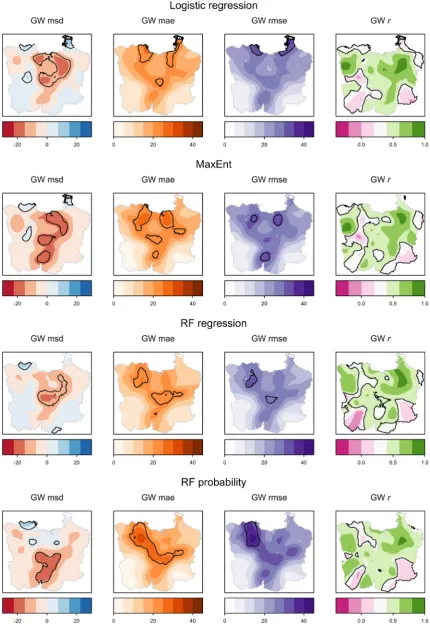
Fig. 6maps the three GW error diagnostics and GWrin the four AGB datasets. Rodríguez-Veiga’s dataset shows relatively small spatial variation in these diagnostics whilst Hu’s dataset shows the largest variation. All four datasets perform very differently to each other with little spatial correspondence in their error.

In Rodríguez-Veiga’s dataset, there is a‘significant’cluster of posi-tive values of GW msd in the dry forests of the North-West, which is coupled with relatively small GW mae and GW rmse values and positive GWrvalues. Forests in this area are often utilized for slash-and-burn

agriculture, and the re-growth of trees can influence the remote sensing signals, resulting in potentially large prediction errors, but where it appears, not so large to adversely influence GW mae, and GW rmse, and GWr. Conversely, there are‘significant’clusters of negative values of GW msd in the moist forests of central-Eastern areas. These areas are coupled with‘significant’clusters of relatively large GW mae and GW rmse values and a‘significant’cluster of negative GWrvalues. Thus, this dataset clearly performs worse in central-Eastern areas, as all four GW diagnostics indicate so. In this central-Eastern area, the forest is matured with large AGBs, so the saturation of spectral data from sa-tellite sensors may be a cause of the inaccurate predictions.

Baccini’s dataset depicts a‘significant’cluster of large positive GW msd values in the south, where the same area provides‘significantly’ large GW mae, and GW rmse values, all suggesting an area of relatively poor AGB accuracy. Of note is the spatial behavior of GW r, where ‘significant’negative correlations are of concern. Such clusters occur in quite different areas to the cluster observed in south for unusually large GW mae, and GW rmse values. Similar to thefirst case study, GWr provides an alternative assessment of local error to GW mae and GW rmse. A possible explanation for this, is that GWrcan be sensitive to bandwidth size. For example, a few anomalous pairs of predicted and reference data points that fall close to the kernel centre can exert an undue influence on the correlation estimate (see Section5). In com-parison to Rodríguez-Veiga’s dataset, Baccini’s dataset consistently performs worse in terms of AGB accuracy except a small portion of the central region in terms of GW mae.

Saatchi’s dataset is relatively accurate in central areas with small GW msd, GW mae, and GW rmse values, whilst it is the least accurate the South-West, as confirmed by the permutation tests for GW msd, GW mae, and GW rmse, where‘significantly’large values are found. The GWrmap shows negative values in many regions, but where no ‘sig-nificant’ clusters of this diagnostic are found. In comparison to Rodríguez-Veiga’s dataset, Saatchi’s dataset appears to perform better in some central-Eastern areas in terms of GW mae.

Hu’s dataset depicts very different spatial patterns of the GW diag-nostics to the other three datasets, and is clearly the least accurate with over-prediction almost everywhere. In particular,‘significantly’large GW msd, GW mae, and GW rmse values can be found in North-Eastern areas. A‘significantly’large negative GWrvalues are observed in the south but different areas from other three GW diagnostics.

In summary, mapping GW diagnostics provides useful spatial in-dications of the reliability of each dataset, not only individually, but also in comparison with each other. Despite all four datasets depicting the same AGB measure, the spatial patterns of error and accuracy vary in each dataset. Rodríguez-Veiga’s dataset would be the best choice in terms of the conventional diagnostics (Table 3), but not necessarily the best choice everywhere, for example in central-Eastern areas, where Saatchii’s dataset may be more accurate and preferred.

5. Discussion

The use of GW diagnostics has allowed investigations of the spatial structure of error between predicted and reference values for two EO case studies. This approach extends conventional (single-valued) whole map diagnostics of error spatially, through their localized (multiple-valued) counterparts. The associated permutation tests can highlight unusually accurate or unusually inaccurate error, providing a means to focus EO or other research activity on specific areas. This work is novel, but a number of points warrant discussion.

5.1. The effects of sample information

In this study, the use of the same reference data to evaluate the GW diagnostics of different datasets ensures results are comparable. However, an independent reference sample is not always available. This is a limitation for any error assessment: any results are only ever Table 3

Global diagnostics and Moran’sIin forest aboveground biomass datasets for study 2.

msd mae rmse r Moran’sI* Rodríguez-Veiga et al. −2.05 31.52 39.42 0.50 0.08 Baccini et al. −86.36 89.10 105.58 0.36 0.35 Saatchi et al. −45.26 58.78 70.69 0.08 0.29 Hu et al. −136.35 141.76 153.75 0.36 0.24

* Allp-values for estimates of Moran’sIare less than 0.05.

relative to the reference sample. For case study 2, Rodríguez-Veiga’s dataset yielded the most accurate AGB performance amongst the four AGB datasets in most parts of the study area. The reference sample used here, despite being independent from the training data used for the

reference data than the other datasets with spatial resolutions of 500 m or 1 km. Such characteristics need to be accounted for when comparing continuous raster datasets.

5.2. Bandwidth specification

In this work, a user-specified bandwidth of 10% was used for all outputs. This in part, reflected the need to use only one bandwidth throughout, so that multiple datasets could objectively be compared. However, in any GW approaches, the selection of the bandwidth is critical, to identify which levels of spatial heterogeneity should be fo-cused. For example,Fig. 7shows the results of generating GW mae for Saatchi’s dataset in case study 2, with a range of adaptive bandwidth sizes (5%–50% in increments of 5%). Small bandwidth sizes result in highly localized variations in GW mae, while larger bandwidths result in a greater degree of smoothing and tend to be the global mae of 58.78 Mg ha−1. Thus, results and interpretations are dependent on the user-specified 10% bandwidth. This can be overcome by calculating and visualizing a series of GW diagnostics over a range of bandwidths as an exploratory step. Although objective bandwidth selection proce-dures are available (Gollini et al., 2015;Harris et al., 2014), their use commonly results in one ‘best on average’ bandwidth choice that maximizes the precision of the predictor or statistic (e.g. via a leave-one-out cross-validation). Such data-driven procedures should not be regarded as a panacea for bandwidth selection or the degree of smoothing to use (Ruppert et al., 1995).

5.3. The difference between mae and rmse

It is important to acknowledge the difference between mae and rmse, which is often over-looked. The mae represents average error magnitude (averaged absolute error) (Willmott and Matsuura, 2005), and rmse reflects the mean and variation in the error and is therefore highly sensitive to outliers (Pontius et al., 2008; Willmott and Matsuura, 2005). In this sense, mapping GW mae captures the spatial variation of the average error magnitude, whilst GW rmse highlights larger errors compared to GW mae. This is originated from the fact that the mean squared error, which is the squared rmse, is composed of the squared msd and the variance (Friedman, 1997). Because of this char-acteristic, rmse has no clear interpretation, unlike mae. A GW-based extension of such discussions would be an interesting topic of future work.

6. Conclusions

Conventional diagnostics of error, such as msd, mae and rmse pro-vide global,‘on-average’measures. These summary measures of error do not capture any spatial information of the error. Ignoring spatial structures in error may result in a false interpretation and misuse of the data that the errors stem from. This work develops and applies localized diagnostics of error to investigate spatial heterogeneity of each types of these diagnostics. Two case studies demonstrate their value for com-paring multiple models and for comcom-paring multiple datasets. Comparing multiple models can support a deeper understanding of the spatial characteristics of errors and in turn can inform analytical choices and data collection to improve data accuracy and reliability. Identifying distinct local error clusters can help focus efforts in this respect. When multiple datasets are compared, understanding the spa-tial distributions of error in different datasets can inform choices about which datasets to use and in which areas to use them.

Acknowledgements

We appreciate anonymous reviewers for giving insightful com-ments. This research is funded by KAKENHI Grant Number 15K21086; KU SPIRITS project; ROIS-DS-JOINT (006RP2018); and joint research program of CEReS, Chiba university(2018). P. Rodríguez Veiga and H. Balzter were supported by the UK’s National Centre for Earth Observation (NCEO). A. Comber and P. Harris were supported by the Natural Environment Research Council Newton Fund grant (NE/ N007433/1). We thank M. Castillo, I. Cruz, and M. Olguin for giving advice on the Mexican case study. All statistical analyses and mapping were conducted in the R open source software. Functions to calculate GW mae and GW rmse and their Monte Carlo permutation tests re-quired a series of adaptions to the functionsgwssandgwss.montecarloin the GWmodel R package (Gollini et al., 2015;Lu et al., 2014). These adapted functions are available to interested researchers on request. Options for GW msd and GWrand their tests are already provided in the same functions of the GWmodel.

References

Baccini, A., Goetz, S.J., Walker, W.S., Laporte, N.T., Sun, M., Sulla-Menashe, D., Hackler, J., Beck, P.S.A., Dubayah, R., Friedl, M.A., Samanta, S., Houghton, R.A., 2012. Estimated carbon dioxide emissions from tropical deforestation improved by carbon-density maps. Nat. Clim. Change 2, 182–185.https://doi.org/10.1038/

nclimate1354.

Breiman, L., 2001. Random forests. Mach. Learn. 45, 5–32.https://doi.org/10.1023/ A:1010933404324.

Fig. 7.Comparison of results of GW mae for Saatchi’s aboveground biomass dataset with different adaptive kernel size between 5%–50% as an example.

Brunsdon, C., Fotheringham, A.S., Charlton, M.E., 1996. Geographically Weighted Regression: A Method for Exploring Spatial Nonstationarity. Geogr. Anal. 28, 281–298.https://doi.org/10.1111/j.1538-4632.1996.tb00936.x.

Brunsdon, C., Fotheringham, A.S., Charlton, M., 2002. Geographically weighted summary statistics—a framework for localised exploratory data analysis. Comput. Environ. Urban Syst. 26, 501–524.

Comber, A.J., 2013. Geographically weighted methods for estimating local surfaces of overall, user and producer accuracies. Remote Sens. Lett. 4, 373–380.https://doi. org/10.1080/2150704X.2012.736694.

Comber, A.J., Fisher, P., Brunsdon, C., Khmag, A., 2012. Spatial analysis of remote sen-sing image classification accuracy. Remote Sens. Environ. 127, 237–246.https://doi. org/10.1016/j.rse.2012.09.005.

Comber, A., See, L., Fritz, S., Van der Velde, M., Perger, C., Foody, G.M., 2013. Using control data to determine the reliability of volunteered geographic information about land cover. Int. J. Appl. Earth Obs. Geoinf. 23, 37–48.https://doi.org/10.1016/j.jag. 2012.11.002.

Comber, A.J., Harris, P., Tsutsumida, N., 2016. Improving land cover classification using input variables derived from a geographically weighted principal components ana-lysis. ISPRS J. Photogramm. Remote Sens. 119, 347–360.https://doi.org/10.1016/j. isprsjprs.2016.06.014.

Comber, A., Brunsdon, C., Charlton, M., Harris, P., 2017. Geographically weighted cor-respondence matrices for local error reporting and change analyses: mapping the spatial distribution of errors and change. Remote Sens. Lett. 8, 234–243.https://doi. org/10.1080/2150704X.2016.1258126.

Congalton, R.G., 1988. Using spatial autocorrelation analysis to explore the errors in maps generated from remotely sensed data. Photogramm. Eng. Remote Sens. 54, 587–592.

Congalton, R.G., 1991. A review of assessing the accuracy of classifications of remotely sensed data. Remote Sens. Environ. 37, 35–46. https://doi.org/10.1016/0034-4257(91)90048-B.

Daly, C., 2006. Guidelines for assessing the suitability of spatial climate data sets. Int. J. Climatol. 26, 707–721.https://doi.org/10.1002/joc.1322.

Foody, G.M., 2002. Status of land cover classification accuracy assessment. Remote Sens. Environ. 80, 185–201.https://doi.org/10.1016/S0034-4257(01)00295-4. Foody, G.M., 2005. Local characterization of thematic classification accuracy through

spatially constrained confusion matrices. Int. J. Remote Sens. 26, 1217–1228.

https://doi.org/10.1080/01431160512331326521.

Fotheringham, A.S., Brunsdon, C., Charlton, M., 2002. Geographically Weighted Regression: The Analysis of Spatially Varying Relationships. Wiley, Chichester. Friedman, J.H., 1997. On bias, variance, 0/1-loss, and the curse-of-dimensionality. Data

Min. Knowl. Discov. 1, 55–77.https://doi.org/10.1023/A:1009778005914. Gollini, I., Lu, B., Charlton, M., Brunsdon, C., Harris, P., 2015. GWmodel : An R Package

for Exploring Spatial Heterogeneity Using Geographically Weighted Models. J. Stat. Softw. 63, 85–101.https://doi.org/10.18637/jss.v063.i17.

Harris, P., Brunsdon, C., 2010. Exploring spatial variation and spatial relationships in a freshwater acidification critical load data set for Great Britain using geographically weighted summary statistics. Comput. Geosci. 36, 54–70.https://doi.org/10.1016/j. cageo.2009.04.012.

Harris, P., Juggins, S., 2011. Estimating freshwater acidification critical load exceedance data for great britain using space-varying relationship models. Math. Geosci. 43, 265–292.https://doi.org/10.1007/s11004-011-9331-z.

Harris, P., Brunsdon, C., Charlton, M., 2013. The comap as a diagnostic tool for non-stationary kriging models. Int. J. Geogr. Inf. Sci. 27, 511–541.https://doi.org/10.

1080/13658816.2012.698014.

Harris, P., Clarke, A., Juggins, S., Brunsdon, C., Charlton, M., 2014. Geographically weighted methods and their use in network re-designs for environmental monitoring. Stoch. Environ. Res. Risk Assess. 28, 1869–1887. https://doi.org/10.1007/s00477-014-0851-1.

Hu, T., Su, Y., Xue, B., Liu, J., Zhao, X., Fang, J., Guo, Q., 2016. Mapping Global Forest Aboveground Biomass with Spaceborne LiDAR, Optical Imagery, and Forest Inventory Data. Remote Sens. (Basel) 8, 565.https://doi.org/10.3390/rs8070565. Khatami, R., Mountrakis, G., Stehman, S.V., 2017. Predicting individual pixel error in remote sensing soft classification. Remote Sens. Environ. 199, 401–414.https://doi. org/10.1016/j.rse.2017.07.028.

Liu, C., Frazier, P., Kumar, L., 2007. Comparative assessment of the measures of thematic classification accuracy. Remote Sens. Environ. 107, 606–616.https://doi.org/10. 1016/j.rse.2006.10.010.

Lu, B., Harris, P., Charlton, M., Brunsdon, C., 2014. The GWmodel R package: further topics for exploring spatial heterogeneity using geographically weighted models. Geo. Inf. Sci. 17, 85–101.https://doi.org/10.1080/10095020.2014.917453. Monteys, X., Harris, P., Caloca, S., Cahalane, C., 2015. Spatial prediction of coastal

bathymetry based on multispectral satellite imagery and multibeam data. Remote Sens. 7, 13782–13806.https://doi.org/10.3390/rs71013782.

Phillips, S.J., Dudík, M., 2008. Modeling of species distribution with Maxent: new ex-tensions and a comprehensive evaluation. Ecograpy 31, 161–175.https://doi.org/10. 1111/j.2007.0906-7590.05203.x.

Pontius, R.G., Thontteh, O., Chen, H., 2008. Components of information for multiple resolution comparison between maps that share a real variable. Environ. Ecol. Stat. 15, 111–142.https://doi.org/10.1007/s10651-007-0043-y.

Rodríguez-Veiga, P., Saatchi, S., Tansey, K., Balzter, H., 2016. Magnitude, spatial dis-tribution and uncertainty of forest biomass stocks in Mexico. Remote Sens. Environ. 183, 265–281.https://doi.org/10.1016/j.rse.2016.06.004.

Ruppert, A.D., Sheather, S.J., Wand, M.P., 1995. An effective bandwidth selector for local least squares regression. J. Am. Stat. Assoc. 90, 1257–1270.

Saatchi, S.S., Harris, N.L., Brown, S., Lefsky, M., Mitchard, E.T.A., Salas, W., 2011. Benchmark map of forest carbon stocks in tropical regions across three continents. Proc. Natl. Acad. Sci. U. S. A. 108.https://doi.org/10.1073/pnas.1019576108. See, L., Perger, C., Hofer, M., Weichselbaum, J., Dresel, C., Fritz, S., 2015. Laco-Wiki: an

Open Access Online Portal for Land Cover Validation. ISPRS Ann. Photogramm. Remote Sens. Spat. Inf. Sci. II-3/W5, 167–171. https://doi.org/10.5194/isprsannals-II-3-W5-167-2015.

Stehman, S.V., Czaplewski, R.L., 1998. Design and analysis for thematic map accuracy assessment. Remote Sens. Environ. 64, 331–344. https://doi.org/10.1016/S0034-4257(98)00010-8.

Tsutsumida, N., Comber, A.J., 2015. Measures of spatio-temporal accuracy for time series land cover data. Int. J. Appl. Earth Obs. Geoinf. 41, 46–55.https://doi.org/10.1016/ j.jag.2015.04.018.

Tsutsumida, N., Comber, A., Barrett, K., Saizen, I., Rustiadi, E., 2016. Sub-pixel classifi -cation of MODIS EVI for annual mappings of impervious surface areas. Remote Sens. 8, 143.https://doi.org/10.3390/rs8020143.

Willmott, C., Matsuura, K., 2005. Advantages of the mean absolute error (MAE) over the root mean square error (RMSE) in assessing average model performance. Clim. Chang. Res. Lett. 30, 79–82.https://doi.org/10.3354/cr030079.

Willmott, C.J., Matsuura, K., 2006. On the use of dimensioned measures of error to evaluate the performance of spatial interpolators. Int. J. Geogr. Inf. Sci. 20, 89–102.