EXPLAINING TRAFFIC FLOW PATTERNS USING CENTRALITY
MEASURES
Amila Jayasinghe1, Kazushi Sano2, Hiroaki Nishiuchi3
1, 2, 3 Urban Transport Engineering and Planning Lab, Department of Civil and Environmental
Engineering, Environment Systems Engineering, Graduate School of Engineering - Doctoral Program, Nagaoka University of Technology, Nagaoka, 940-2137, Japan
Received 6 January 2015; accepted 21 April 2015
Abstract: This study examines the capability of centrality parameters of the road network to explain and predict traffic flow by types of vehicles. The case study was conducted in Colombo Metropolitan Area, Sri Lanka. Study used four centrality parameters i.e. connectivity, global integration, local integration and choice; and three analysis methods i.e. topological, metric and angular which introduced by space syntax analysis method to compute network centrality of the road network. Findings of this study stress that, (1) human beings perceive the space mostly from geometrical distance (topological and angular distance) in comparison to metric distance. Further to this, it was found that angular distance is more powerful in global level whereas topological distance is more powerful in local level; (2) it is more appropriate to consider the multiple influences from multiple centrality parameters rather being confined to a single best parameter and influence of each parameter varies based on type of vehicles. Keywords: traffic volume by type of vehicles, network centrality, space syntax.
1 Corresponding author: [email protected]
1. Introduction
Rapid increase of vehicle movements has created several problems such as traffic congestion, road accidents and air pollution in urban areas. Accordingly, identification of locations which attract more traffic and finding out reasons for that; and prediction of future traffic flow scenarios based on proposed transport networks and land use changes are some important tasks that most of the practitioners and researchers in traffic and transport engineering and planning as well as in urban planning and spatial design are involved the most. This understanding guides traffic and transport engineers and planners to resolve many burning issues
highlighted the importance of considering the road network geometry and topology in the process of modeling or simulating traffic flow patterns.
Those studies are focused on an emerging set of research literature which is developed based on the graph theory and centrality measures. Accordingly, the group of scholars in London led by Bill Hillier (Hillier and Hanson, 1984), (Hillier, 1999) mapped the centrality in cities under the notion of space syntax. In space syntax, centrality was termed as ‘integration’ and mapped as a property topology of the space on an index of closeness or accessibility and it recognized that human movements are related to the level of integration of a given Road network (Hillier, 1999). Porta et al. (2006) have introduced Multiple Centrality Assessment (MCA), MCA application measures the level that a given location is “being central” not only through the means of being close to all others (i.e. Closeness), but also through the means of being intermediary between others (i.e. Betweenness), being straight to all others (i.e. Straightness) and being critical for the efficiency of the system as a whole (Porta et al., 2006). Those researches provided the back bone to a wide spectrum of options on the use of centrality measures to explain and predict human and vehicular traffic flow. Jun et al. (2007) used ‘depth’ (weighted syntax based on O-D trips) centrality measure in space syntax to model the number of transfers in the journey of rail, tram, and bus routes in Seoul city, Korea. Scheurer et al. (2007) identified and visualized the strengths and weaknesses of public transport networks, in terms of geographical coverage, network connectivity, competitive speed and service
levels, by using multiple centrality measures i.e. degree centrality, closeness centrality and betweenness centrality in urban public transport networks of Australian cities (Perth, Melbourne). Kazerani and Stephanr (2009) used modified version of betweenness centrality and studied dynamics and temporal aspects of people’s travel demand in CBD area. Jiang and Jia (2011) explored complex collective human movement behaviors in geographic space and what kind of useful patterns or knowledge can discover from using network centrality with agent-based simulation based on London street network. Altshuler et al. (2011) used augmented betweenness centrality measure for mobility prediction in transportation networks based on Israeli roads and highways system.
In that background, this research attempted to constructively contribute in overcoming one of the key limitation noted in the above mentioned emerging research in relation to traffic and transport engineering and panning domain. That is, those studies have been focused on total traffic volume or one mode of traffic rather compare and contrast the characteristics of traffic flow pattern by type of vehicle (i.e. motor cycles, three wheeler, cars, bus, heavy vehicle etc.) in relation to centrality measures. Addressing the above gap, this study attempted to explain the predominant road network centrality characteristics that attract more vehicular traffic by type of vehicle using road network of the Colombo Metropolitan Area (CMA), Sri Lanka.
about the study area. Analysis and results describe in the section three. Conclusions and recommendations for future studies then follow in section four.
2. Methodology
T he st udy conduc ted i n Colombo Metropolitan Area (CMA) which is the main urban agglomeration area in Sri Lanka. CMA is one of the emerging urban
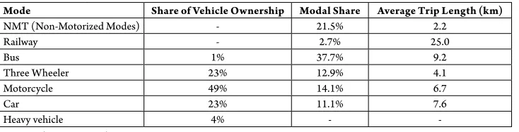
agglomerations in south Asia with 5.8 million residential population (30% of the country population) and it account 50% of country’s GDP (Department of Census & Statistics, 2012). The per capita trip rate is recorded as 1.87 per person (JICA, 2014) and around 700,000 trips are generated within the CMA area (JICA, 2014). Table 1 gives a brief description about the traffic and transport characteristics of CMA area.
Table 1
Traffic and Transport Characteristics of CMA Area
Mode Share of Vehicle Ownership Modal Share Average Trip Length (km)
NMT (Non-Motorized Modes) - 21.5% 2.2
Railway - 2.7% 25.0
Bus 1% 37.7% 9.2
Three Wheeler 23% 12.9% 4.1
Motorcycle 49% 14.1% 6.7
Car 23% 11.1% 7.6
Heavy vehicle 4% -
-Source: (JICA, 2014)
The study comprised of three main steps. The first was the preparation of a GIS database. The second was the ‘Network Centrality Assessment’ (NCA). The third was to investigate a possible relationship between the network centrality and actual vehicle traffic volumes.
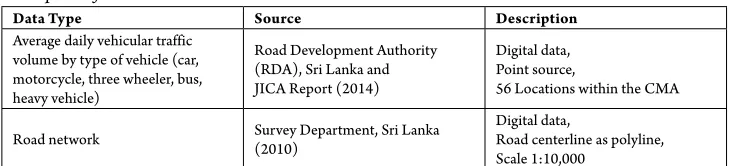
2.1. Stage 1 - Preparation of the GIS
Database
Table 2
Description of GIS Database
Data Type Source Description
Average daily vehicular traffic volume by type of vehicle (car, motorcycle, three wheeler, bus, heavy vehicle)
Road Development Authority (RDA), Sri Lanka and JICA Report (2014)
Digital data, Point source,
56 Locations within the CMA
Road network Survey Department, Sri Lanka (2010) Digital data, Road centerline as polyline, Scale 1:10,000
2.2. Stage 2 - Network Centrality
Assessment (NCA)
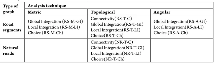
The method used for NCA in this study was based on the space syntax approach. This study used two types of graphs; ‘axial segments’ (this will be referred as ‘road segments’ in rest of the paper) and ‘natural roads’ to represent road networks. Metric, topological and angular (geo-metrical) analysis techniques are employed to compute network centrality based on connectivity, global integration, local integration and choice centrality parameters. Refer Fig. 1 for more details.
Initial step of the NCA was preparation of a graph based on the real road network. Accordingly, two types of graphs (i.e. road segments graph and natural roads graph) were prepared in this study. Refer step-1 in Fig. 1 for more details. Preparation of the road segments graph followed the method which is introduced by Turner (2001) and it enabled the angular analysis technique of space syntax. Accordingly, centerlines of road network were used and in order to prepare the road segments graph, each road centerline was broken at the intersection (i.e. the place where two or more centerlines meet). To do that,
coverage file creation option of ArcGIS 10.0 was used. Preparation of natural roads graph is followed the method which is introduced by Jiang and Liu (2009). Accordingly, Axwoman extension in ArcGIS 10.0 was employed to create natural roads graph by tracking the road segments in the road segments graph. 45 degree was considered as the angle change limitation value.
Using those graphs, centralities of each link were calculated based on (1) Connective centrality (Ci); the level of Ci refers the
number of links to which the particular link is directly connected in the graph, (2) Global Integration (GIi); level of GIirefers
the extent that given link close to all other links in the graph, (3) Local Integration (LIi); level of LIi refers the extent that given
link close to all other links in radius of 3 or 7 steps away from it, and (4) Choice (Chi);
level of choice is refers the extent a given link belongs to the shortest-path between any pairs of two links in the graph. Refer step-2 centrality parameters subsection in Fig. 1 for more details. Accordingly, centrality of links in road segments graph
was computed based on three analysis techniques by using UCL Depth Map 10 software application. However, centrality of links in natural roads was computed only based on topological analysis method due to the limited functions of software (Axwoman extension in ArcGIS and Pajek software applications). Refer step-2 in Fig. 1 for more details.
Finally, those outputs were spatially joined and created the centrality index. The centrality index is comprised with centrality values according to the 14 different parameters, spatial coordinates and reference ID number of each links. Refer step-3 in Fig. 1 for more details.
Table 3
Centrality Combinations Calculated under the NCA Type of
graph
Analysis technique
Metric Topological Angular
Road segments
Global Integration (RS-M-GI) Local Integration (RS-M-LI) Choice (RS-M-Ch)
Connectivity(RS-T-C) Global Integration(RS-T-GI) Local Integration(RS-T-LI) Choice(RS-T-Ch)
Global Integration(RS-A-GI) Local Integration(RS-A-LI) Choice (RS-A-Ch)
Natural roads
Fig. 1.
2.3. Stage 3 - Relationship Analysis
The third stage was to investigate if any possible relationships exists between the network centrality and actual vehicle traffic volumes. The ‘Centrality Index’ and ‘Vehicular Traffic Index’, which include information related to average daily vehicular traffic by type of vehicles, were compared to recognize relationships. The analysis was carried at two levels. First, bivariate pearson correlation coefficient test in SPSS (Statistical Package for Social Science, 18th version) software was employed to find out the nature and the strength of a relationship between different centrality values and vehicular traffic volume by type of vehicle. Then, forward multiple regression analysis was employed to identify cumulative impact from different centrality parameters on
vehicular traffic by type of vehicles. A quasi-hedonic model explaining the vehicular traffic volume by type of vehicles taking the following form is going to be created, tested, and analyzed in multiple regression.
Vehicular traffic volume by mode i =
ƒ(RS-M-GI . RS-M-LI . RS-M-Ch . RS-T-C . RS-T-GI . RS-T-LI . RS-T-Ch . RS-A-GI . RS-A-LI . RS-A-Ch . NR-T-C . NR-T-GI . NR-T-LI . NR-T-Ch)
Results of those two analyses are summarized in next section.
3. Analysis and Inferences
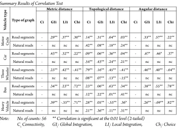
Table 4 illustrates the summary of the result reveled from correlation analysis.
Table 4
Summary Results of Correlation Test
Ve
hi
cl
e t
yp
e
Type of graph
Metric distance Topological distance Angular distance
Ci GIi LIi Chi Ci GIi LIi Chi Ci GIi LIi Chi
M
ot
or
C
ycle Road segments - .29** .37** .30** .14** .31** .64** .03** - .33** .57** .22**
Natural roads - nc nc nc .42** .08** .18** .24** - nc nc nc
Ca
r Road segments - .43** .32** .22** .09** .06** .36** .04** - .67* .46* .37*
Natural roads - nc nc nc .54** .43** .24** .21** - nc nc nc
T
hr
ee
W
he
ele
r Road segments - .23** .42** -.41** .79** .16** .45** -.41** - .46** .40** -.64**
Natural roads - nc nc nc .08** .07** .13** -.15** - nc nc nc
Bu
s Road segments - .34** .23** .72** .23** .06** .63** .34** - .38** .55** .78**
Natural roads - nc nc nc .12** .22** .01** .41** - nc nc nc
He
av
y
Ve
hicle Road segments - .39** -.33** .71** .28** .05** -.53** .36* - .26** -.69** .82**
Natural roads - nc nc nc .21** .36** .11** .31** - nc nc nc
Note: No. of counts: 56 ** Correlation is significant at the 0.01 level (2-tailed)
3.1. Correlation Results - Motor Cycle
Traffic Volume and Centrality Values
Significant correlations were found between daily motor cycle traffic volume and centrality values. Centrality values computed based on angular distance and topological distance revealed a highly significant
correlation level than the same of the metric distance. The highest correlation is found with ‘road segments - topological distance - local integration’ (r = 0.64, p < .01) followed by ‘road segments - angular distant - local integration’ (r = 0.57, p < .01), and ‘natural roads - topological distance - connectivity’ (r = 0.42, p < .01).
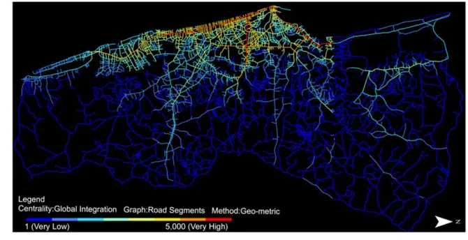
Fig. 2.
The Map Depicts the Spatial Distribution of ‘Road Segments - Topological Distance - Local Integration Centrality’ Values. The Highest Values are Indicated in Red Colour and the Lowest Values are Indicated in Blue Colour
Fig. 3.
3.2. Correlation Results - Car Traffic
Volume and Centrality Values
Centrality values which computed based on angular distance indicated a significant correlation level compare to topological
distance and metric distance. The highest correlation is found with ‘road segments - angular distance - global integration’(r = 0.67, p < .01) followed by ‘natural roads - topological distance - connectivity’ (r = 0.54, p < .01).
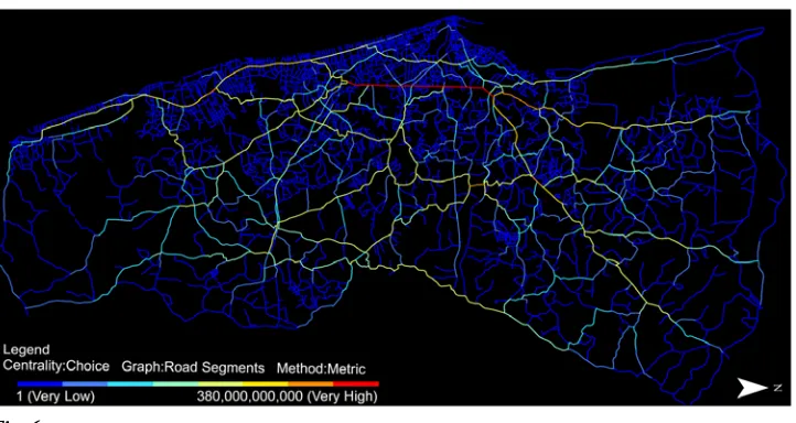
Fig. 4.
The Map Depicts the Spatial Distribution of ‘Road Segments - Angular Distance (Geo-Metric) - Global Integration’ Centrality Values. The Highest Values are Indicated in Red Colour and the Lowest Values are Indicated in Blue Colour
Fig. 5.
3.3. Correlation Results - Three Wheelers
Traffic Volume and Centrality Values
Three wheelers are the most popular taxi service in the study area for short distance (2-5km) trips. ‘Road segments -topological distance - local integration’ revealed a highly significant positive coefficient of correlation (r = 0.79, p < .01) while ‘road segments - angular distance - choice’ revealed a significant negative coefficient of correlation (r = -0.64, p < .01) compare to other. Similar kind of relationship (i.e. positive correlation with local integration and negative correlation with choice) was observed in road segments of both metric
distance and topological distance though their coefficient of correlation values were comparatively low.
3.4. Correlation Results - Bus Traffic
Volume and Centrality Values
It is observed that ‘road segments - angular distance - choice’ (r = 0.78, p < .01) and ‘road segments - metric distance - choice’ (r = 0.72, p < .01) have higher coefficient of correlation values and significant positive correlation with ‘road segments - topological distance - local integration’ (r = 0.63, p < .01) and ‘road segments - angular distance - local integration’ (r = 0.55, p < .01).
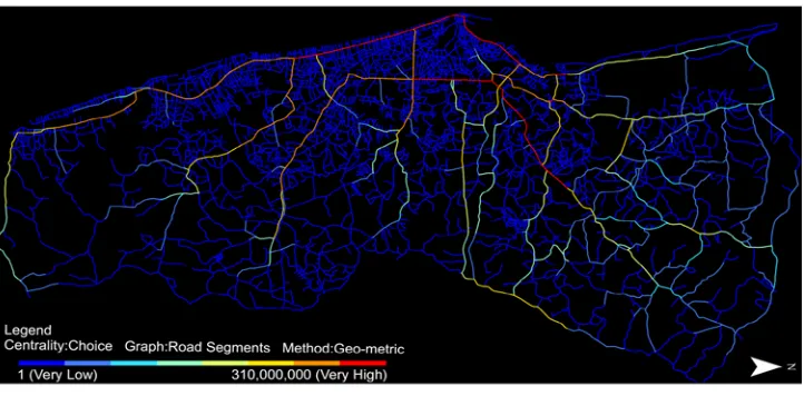
Fig. 6.
Fig. 7.
The Map Depicts the Spatial Distribution of ‘Road Segments - Angular Distance (Geo-Metric) - Choice’ Centrality Values. The Highest Values are Indicated in Red Colour and the Lowest Values are Indicated in Blue Colour
3.5. Correlation Results - Heavy Vehicles
Traffic Volume and Centrality Values
Heavy vehicles are pre dominantly used in transport activities related to Colombo sea port, industrial zones, manufacturing industries, whole-sale and commercial business in the study area. Centrality values computed based on angular distance and metric distance indicated a significant correlation level in comparison to topological distance. Future, ‘road segments - angular distance - choice’ (r = 0.82, p < .01) and ‘road segments - metric distance - choice’ (r = 0.71, p < .01) revealed a highly significant positive coefficient of correlation while ‘road segments - angular distance - local integration’ (r = -0.69, p < .01) and ‘road segments - topological distance - local integration’ (r = -0.53, p < .01) revealed a significant negative coefficient of correlation with heavy vehicle traffic volume.
3.6. Multiple Regression Results - Heavy
Vehicles Traffic Volume and Centrality
Values
Table 5
Summary Results of Multiple Regression Analysis
Ty
pe o
f
Ve
hi
cl
e
Model R-Square Sig. F Change
Correlations Collinearity Statistics
Zero-order Partial (Partial)2% Part (Part)2% Tolerance VIF
M
ot
or
C
yc
le (Constant)
0.627 0.000
RS_T_LI 0.415 0.694 48.2% 0.556 30.9% 0.599 1.669
NR_T_C 0.413 0.237 5.6% 0.144 2.1% 0.748 1.337
RS_A_GI 0.399 0.499 24.9% 0.370 13.7% 0.587 1.704
Ca
r
(Constant)
0.726 0.000
RS_T_LI 0.625 0.494 24.4% 0.372 13.8% 0.625 1.600
NR_T_C 0.467 0.212 4.5% 0.133 1.8% 0.724 1.381
RS_A_Ch 0.04 0.447 20.0% 0.341 11.6% 0.623 1.605
RS_A_GI 0.679 0.668 44.7% 0.494 24.4% 0.679 1.473
T
hr
ee
W
he
ele
r (Constant)
0.685 0.000
RS_T_LI 0.679 0.737 54.3% 0.524 27.5% 0.679 1.473
RS_A_Ch 0.071 -0.483 23.3% -0.368 13.5% 0.610 1.639
RS_A_GI 0.513 0.326 10.6% 0.278 7.7% 0.601 1.664
Bu
s
(Constant)
0.794 0.000
RS_A_Ch 0.679 0.717 51.4% 0.494 24.4% 0.679 1.473
RS_T_LI 0.625 0.602 36.2% 0.372 13.8% 0.625 1.600
RS_A_LI 0.497 0.308 9.5% 0.147 2.2% 0.597 1.675
RS_A_GI 0.448 0.351 12.3% 0.299 8.9% 0.548 1.825
H
eav
y V
eh
ic
le
s (Constant)
0.778 0.000
RS_A_Ch 0.729 0.704 49.6% 0.517 26.7% 0.585 1.709
RS_A_LI 0.215 -0.532 28.3% -0.432 18.7% 0.567 1.764
RS_A_GI 0.634 0.432 18.7% 0.369 13.6% 0.571 1.751
Note: RS: Road segments graph, NR: Natural roads graph, A: Angular distance, T: Topological distance, C: Connectivity, GI: Global Integration, LI: Local Integration, Ch: Choice
Results indicated that 63% (R-square 0.627, p < .001) of motor cycle vehicular traffic can be explained by ‘road segments - topological distance - local integration’ (RS_T_LI), ‘natural roads - topological
traffic is influence by RS_T_LI while 24.9% (Partial correlation = 0.499) by RS_A_GI and 5.6% (Partial correlation = 0.237) by NR_T_C.
In related to car vehicular traffic, the multiple regression model with four predictors (i.e. ‘road segments - topological distance - local integration’, ‘natural roads - topological distance - connectivity’, ‘road segments - angular distance - choice’, ‘road segments - angular distance - global integration’ produced 0.726 (p < .001) of R-square value. Future partial correlation values indicated that ‘road segments - angular distance - global integration’ has the highest influence (44.7%) while ‘road segments - topological distance - local integration’ (24.4%) and ‘road segments - angular distance - choice’ (20.0%) recorded more than 20% influence over car vehicular traffic.
‘Road segments - topological - local integration’ (RS_T_LI), ‘road segments - angular distance - choice’ (RS_A_Ch) and ‘road segments - angular distance - global integration’ (RS_A_GI) predictors recorded 0.685 (p < .001) of R-square value for three wheeler vehicular traffic. RS_T_LI explained 54.3% of variance in the three wheeler vehicular traffic while RS_A_Ch explained 23.3% and RS_A_GI explained 10.6% variance in the three wheeler vehicular traffic. Further results indicated that strong negative relationship between RS_A_Ch and three wheeler vehicular traffic.
The multiple regression model of the bus vehicular traffic recorded the highest R-square (R2 = 0.794, p < .001) value
compare to other four modes. ‘Road segments - angular distance - choice’ (51.4%) and ‘road segments - topological - local integration’ (36.2%) recorded the
very significant influence on bus vehicular traffic compare to ‘road segments - angular distance - global integration’ (12.3%) and ‘road segments - angular distance - local integration’ (9.5%).
Last model recorded 78% (R-square 0.778, p < .001) predictability between centrality values and heavy vehicular traffic. Accordingly, Road segments - angular distance - choice’ (RS_A_Ch) explains nearly 50% of heavy vehicle traffic while 28.3% by ‘road segments - angular distance - local integration’ (RS_A_LI ) and 18.7% by ‘road segments - angular distance - global integration’ RS_A_GI explains of heavy vehicle traffic.
4. Discussions and Conclusions
The findings of this study on one hand sustain some of the augments put forward by previous studies and on other hand contribute newly on studies related to vehicular traffic and centrality measures. Hillier and Iida (2005) as well as Turner (2001) have found that human beings perceive the space mostly from geometrical distance (topological and angular distance) rather than metric distance. The results of this study too revealed a similar kind relationship, yet, further to this we found that angular distance is more powerful in global level (i.e. global integration and choice) whereas topological distance is more powerful in local level (i.e. local integration and connectivity).
movement data than closeness (similar to integration) centrality parameter (Hillier and Iida, 2005).However, this study found that it is more appropriate to consider the multiple influences from multiple centrality parameters rather being confined to a single best parameter and influence of each parameter varies based on type of vehicles as follows;
• Local integration (positive relationship and level influence aggregately 48% and individual 31%); the level that road segment is located near (in terms of topological distance) to the road segments in the surrounding area, global integration (positive relationship and level influence aggregately 25% and individual 14%); the level that road segment is located near (in terms of angular distance) to the road segments in the region, and connectivity (positive relationship and level inf luence aggregately 6% and individual 2%); the level that road is directly connected to the other roads in the region are key centrality parameters in relations to moto cycle vehicular traffic.
• Global integration (positive relationship and level influence aggregately 45% and individual 25%); the level that road segment is located near (in terms of angular distance) to the road segments in the region, local integration (positive relationship and level inf luence aggregately 25% and individual 14%); the level that road segment is located near (in terms of topological distance) to the road segments in the surrounding area; choice (positive relationship and level influence aggregately 20% and individual 12%); the level that road segment is located central (or
intermediary) to the shortest paths (in terms of angular distance distance) which links the road segments in the region and connectivity (positive relationship and level inf luence aggregately 5% and individual 2%) ; the level that road is directly connected to the other roads in the region are key centrality parameters in relations to car vehicular traffic.
• Local integration (positive relationship and level influence aggregately 54% and individual 28%); the level that road segment is located near (in terms of topological distance) to the road segments in the surrounding area, choice (negative relationship and level influence aggregately 24% and individual 14%); the level that road segment is located central (or intermediary) to the shortest paths (in terms of angular distance) which links the road segments in the region and global integration (positive relationship and level influence aggregately 11% and individual 8%); the level that road segment is located near (in terms of angular distance) to the road segments in the region are key centrality parameters in relations to three wheeler vehicular traffic.
to the road segments in the surrounding area, local integration (positive relationship and level inf luence aggregately 10% and individual 2%); the level that road segment is located near (in terms of angular distance) to the road segments in the surrounding area and global integration (positive relationship and level inf luence aggregately 12% and individual 9%); the level that road segment is located near (in terms of angular distance) to the road segments in the region are key centrality parameters in relations to bus vehicular traffic.
• Choice (positive relationship and level inf luence aggregately 50% and individual 27%); the level that road segment is located central (or intermediary) to the shortest paths (in terms of angular distance) which links the road segments in the region, global integration (positive relationship and level influence aggregately 19% and individual 14%); the level that road segment is located near (in terms of angular distance) to the road segments in the region and Local integration (negative relationship and level influence aggregately 28% and individual 19%); the level that road segment is located near (in terms of topological distance) to the road segments in the surrounding area are key centrality parameters in relations to heavy vehicular traffic.
With those findings, this study suggests that the influence of network geometry on vehicular traffic could provide a way to enrich traffic and transport models as well as guide transport engineers and planners
in justifying their planning decisions in formulating transportation strategies, plan and policies much more comprehensively. Future studies can further contribute to this through incorporating the track information (including information related to origin, destination, route etc.) of vehicle users.
References
Altshuler, Y.; Puzis, R.; Elovici, Y.; Bekhor, S.; Pentland, A. 2011. Augmented Betweenness Centrality for Mobility Prediction in Transportation Networks.
Athens. In Proceedings of the International Workshop on
Finding Patterns of Human Behaviors in Network and Mobility
Data (NEMO), 1-12.
Chiaradia, A. 2007. Emergent Route Choice Behaviour, Motorway and Trunk Road Network: the Nantes
conurbation. In Proceedings of the 6th International Space
Syntax Symposium, ITU Faculty of Architecture, İstanbul, 078.1-078-17.
Crucittia, P.; Latorab, V.; Marchioric, M. 2004. Topological analysis of the Italian electric power grid, Physica A: Statistical Mechanics and its Applications. DOI:
http://dx.doi.org/10.1016/j.physa.2004.02.029,
338(1-2): 92-97.
Cutini, V. 2001. Configuration and Centrality: Some
evidence from two Italian case studies. In Proceedings
of the 3rd International Space Syntax Symposium, Atlanta, 32.1-32.11.
Department of Census & Statistics, Sri Lanka. 2012.
Census of Population & Housing-2011, Department of
Census & Statistics, Sri Lanka.
Gao, S.; Wang, Y.; Gao, Y.; Liu, Y. 2013. Understanding urban traffic flow characteristics: a rethinking of
betweenness centrality, Environment and Planning B:
Planning and Design. DOI: http://dx.doi.org/10.1068/
b38141, 40(1): 135-153.
Hillier, B. 1999. Space is the Machine: A Configurational
Theory of Architecture. Cambridge: Cambridge University
Press. UK.
Hillier, B.; Hanson, J. 1984. The Social Logic of Space.
Cambridge: Cambridge University Press. UK.
Hillier, B.; Iida, S. 2005. Network and psychological
effects in urban movement. Berlin. In Proceedings of Spatial
Information Theory: International Conference, 475-490.
Holme, P. 2003. Congestion and centrality in traffic
flow on complex networks, Advances in Complex Systems: A
Multidisciplinary Journal. DOI: http://dx.doi.org/10.1142/ S0219525903000803, 6(2): 163-176.
Japan International Cooperation Agency - JICA. 2014. Final Report - CoMTrans Urban Transport Master Plan. Japan International Copperation Agency. Japan.
Jiang, B.; Jia, T. 2011. Agent-based simulation of human movement shaped by the underlying street structure, Journal of Geographical Information Science. DOI: http:// dx.doi.org/10.1080/13658811003712864, 25(1): 51-64.
Jiang, B.; Liu, C. 2009. Street-based topological representations andanalyses for predicting traffic flow in
GIS, International Journal of Geographical Information Science.
DOI: http://dx.doi.org/10.1080/13658810701690448, 23(9): 1119-1137.
Jiang, B.; Yin, J.; Zhao, S. 2014. Characterizing the Human Mobility Pattern in a Large Street Network. Available from Internet: < http://arxiv.org/ftp/arxiv/ papers/0809/0809.5001.pdf >.
Jun, C.; Kwon, J.H.; Choi, Y.; Lee, I. 2007. An Alternative Measure of Public Transport Accessibility Based on
Space Syntax, Advances in Hybrid Information Technology
Lecture Notes in Computer Science. DOI: http://dx.doi.
org/10.1007/978-3-540-77368-9_28, 4413: 281-291.
Kazerani, A.; Stephanr, W. 2009. Modified Betweenness
Centrality for Predicting Traffic Flow. In Proceedings of
the 12th AGILE International Conference, Hannover, 13-21.
Noulas, A.; Scellato, S.; Lambiotte, R.; Pontil, M.; Mascolo, C. 2012. A tale of many cities: universal
patterns in human urban mobility. In PloS one, Public
Library of Science, 7.
Porta, S.; Crucitti, P.; Latora, V. 2006. The network
analysis of urban streets: A dual approach, Physica A.
DOI: http://dx.doi.org/10.1016/j.physa.2005.12.063, 369(2): 853-866.
P u z i s , R . ; A l t s h u l e r , Y . ; E l o v i c i , Y . ; Bek hor, S.; Sh i f ta n, Y.; Pent la nd, A . 2013. Augmented Betweenness Centrality for Environmentally Aware Traffic Monitoring in Transportation Networks, Journal of Intelligent Transportation Systems. DOI: http:// dx.doi.org/10.1080/15472450.2012.716663, 17(1): 91-105.
Scheurer, J.; Curtis, C.; Porta, S. 2007. Spatial Network Analysis of Public Transport Systems: Developing a Strategic Planning Tool to Assess the Congruence of Movement and Urban Structure in Australian Cities. Available from Internet: <http://abp.unimelb.edu.au/ files/miabp/3spatial-network-analysis.pdf>.
Turner, A. 2001. Angular analysis. In Proceedings of the