A NON LINEAR APPROACH TO QUEUEING SYSTEM MODELLING

(1)

A NON LINEAR APPROACH TO

QUEUEING SYSTEM MODELLING

I_{MGBEMENA, CHIKA EDITH*}

Department of Industrial/Production Engineering, Nnamdi Azikiwe University, Awka, Nigeria

2_{MGBEMENA, CHINEDUM OGONNA}

Department of Mechanical Engineering, Nnamdi Azikiwe University , Awka, Nigeria

3_{CHINWUKO EMMANUEL CHUKA}

Department of Industrial/Production Engineering, Nnamdi Azikiwe University, Awka, Nigeria ABSTRACT

This paper seeks to establish queueing models that can help organizations to improve on their customer service within and outside their establishment. New Models were created using non linear regression analysis which is more convenient for the organizations to assess. It was found that The Coefficient of determination, R2_{value equals 1 and} that the Degree of Correlation is 100% which indicates that 100% of the original uncertainty has been explained by the model.

Therefore, the model clearly indicates that the Nonlinear Regression approach can be used to model the queueing system of any organization for improved efficiency.

KEYWORD: Queue, Waiting time, Modelling, Non linear Regression, Organisations.

Nomenclature

s = Number of servers in the queueing system  = Arrival rate.

 = Service rate ρ = Utilization factor

L = Expected number of customers in the queueing system Lq = Expected queue length (excluding customers being served) W = Waiting time in system (includes service time)

Wq = Waiting time in queue

1. Introduction

The behaviour of queueing theory deals with the use of mathematical models to represent the behaviour of customers/clients competing for access to a constrained resource.

(2)

However, the paper was not mathematically exact and therefore the paper “Theory of Probabilities and Telephone Conversations” by A.K Erlang was accepted as the paper with historic importance. Erlang used Probability technique to determine the required number of telephone lines at the Danish Telephone Company.

Special mention should be made of his paper “On the Rational Determination of the Number of Circuits” in which an optimization problem in queueing theory was tackled for the first time [1].

It should be noted that in Erlang’s work, as well as the work done by others in the twenties and thirties, the motivation has been the practical problem of congestion [2,3].

Some of the authors with important contributions are Crommelin, Feller, Jensen, Khintchine, Kolmogorov, Palm, and Pollaczek.

Noting the inadequacy of the equilibrium theory in many queue situations, Pollaczek began investigations of the behavior of the system during a finite time interval. Since then and throughout his career, he did considerable work in the analytical behavioral study of queueing systems [4, 5].

Queueing theory as an identifiable body of literature was essentially defined by the foundational research of the 1950’s and 1960’s [6, 7, 8].

Bailey used generating functions for the differential equations governing the underlying process [9], while Lederman and Reuter used spectral theory in their solution. Laplace transforms were used later for the same problem, and their use together with generating functions has been one of the standard and popular Procedures in the analysis of queueing systems ever since [10].

A probabilistic approach to the analysis was earlier initiated by Kendall when he demonstrated that imbedded Markov chains can be identified in the queue length process in system M/G/1 and GI/M/s. Lindley derived integral equations for waiting time distributions defined at imbedded Markov points in the general queue GI/G/1 [11]. These investigations led to the use of renewal theory in queueing system analysis in the 1960’s. Identification of the imbedded Markov chains also facilitated the use of combinatorial methods by considering the queue length at Markov points as a random walk [12, 13].

Gaver’s analysis of the virtual waiting time of an M/G/1 queue is one of the initial efforts using diffusion approximation for a queueing system. Fluid approximation, as suggested by Newell [14, 15] considers the arrival and departure processes in the system as a fluid flowing in and out of a reservoir, and their properties are derived using applied mathematical techniques [16]. By the end of 1960’s most of the basic queueing systems that could be considered as reasonable models of real world phenomena had been analyzed and the papers coming out dealt with only minor variations of the system without contributing much to methodology.

(3)

Since then, operations researchers trained in mathematical optimization techniques have explored their use in much greater complexity to a large number of queueing systems.

Recently, the queueing system of some banks in Nigeria was modeled by Mgbemena and a queueing management software created in MATLAB which shows at a glance, the behavior of the queueing system and the unit that needs attention at any time [20].

2. Methodologies and Data Gathering The following exercise was performed:

 As clients arrived in an organization, they were given time sheets; these were stamped with the arrival time and then stamped as the clients left each department/unit, this allowed the cycle time for the

department/unit to be calculated. Video data was also taken at various department/units in order to determine service time distributions.

 During the business hour, service times were recorded at each department/unit and queue lengths were recorded periodically. As clients entered the premises, they receive a station visit form, stamped with their arrival time. As they left, they turned in their forms, which were then stamped with a departure time.

Details of this methodology can be seen in [20]. For this study, the queueing system employed is shown below:

Service facility S

S S C C C C C C

C C C Customers

Served Customers Served Customers

Queueing System

Figure 1. Queueing system of an organisation

C = customers

S = servers

3. Mathematical Modeling and Analysis

(4)

The general form of a nonlinear regression model is given by;

f (x) = a0 (1 – e -a

1x) + e (1)

However, the relationship between the non-linear function and data is expressed as: yi = f(ρ; a0, a1) + e = a0 (1 – e -a

1x) + e (2)

 To evaluate the Waiting Time in System W, we make use of the data in the table below:

Table 1: Relationship between independent variables and dependent variable W.

i. S λ. µ x = ρ =

λ/sµ

y = W

1 1 10 6 1.67 15.770

2 2 8 5 0.8 5.6578

3 4 8 7 0.29 5.1279

4 2 10 7 0.71 5.551

5 4 10 9 0.28 5.990

(Source: Data generated from [20])

Here, we use the initial guesses of a0 = 1 and a1 = 1.

The partial derivatives of the function in (1) with respect to the parameters are:

=1- (3) = (4)

But the matrix of the linearized model with respect to the parameters is given by;

[D] = [Zj] [ΔA] + [E] (5)

Where Zj is the matrix of the partial derivatives of the function evaluated at initial guess j;

(6)

(5)

=

0.8118 0.3144 0.5507

0.2517 0.5084 0.2442

0.3594 0.2170 0.3491 0.2116

The matrix multiplied by its transpose gives; [Zo]T _{[Z0] =} 1.4006 0.7589

0.7369 0.4418

Which when inverted yield

[Zo]T _[Z0]-1₌ 7.4188 12.7436 12.3741 23.5191

The vector [D] which consists of the difference between the measurements and the model predictions is given by;

=

14.8292 5.1071 4.8462 5.0426 5.7458

(7)

It is multiplied by [Zo]T _{to give;} [Zo]T ₌ 1.0830

10.5321

The vector ∆ becomes ΔA = 1.5853

0.9412

Which can be added to the initial parameter guesses to yield; 1.0

1.0 + 1.58530.9412 2.58530.0588

Hence, the time the customer spends in the system is related to the independent variables by the formular:

 W = 2.5853(1 – e -0.0588λ/sµ₎ ₍₈₎

 To evaluate the Time spent in queue, we make use of the data in the table below:

Table 2: Relationship between independent variables and dependent variable Wq.

i. s λ. µ x = ρ =

λ/sµ y = Wq

1 1 10 6 1.67 9.809

2 2 8 5 0.8 1.4403

3 4 8 7 0.29 0.00221

4 2 10 7 0.71 0.4345

5 4 10 9 0.28 0.0014

(6)

Also, we use the initial guesses of a0 = 1 and a1 = 1. yields;

8.9272 0.8896 0.2495 0.0739 0.2428

[Zo]T ₌ 8.2022 2.9951 The vector ∆ becomes

ΔA = 0.7088

0.9704

1.0 + 0.70880.9704 1.70880.0296

Hence, the time a customer spends in the queue is related to the independent variables by the formular:

 Wq = 1.7088(1 – e -0.0296λ/sµ₎ ₍₉₎

 To evaluate the Expected Queue Length, we make use of the data in the table below:

Table 3: Relationship between independent variables and dependent variable Lq.

i. s Λ µ x = ρ =

λ/sµ

y = Lq

1 1 10 6 1.67 1.471

2 2 8 5 0.8 0.203

3 4 8 7 0.29 0.00031

4 2 10 7 0.71 0.0416

5 4 10 9 0.28 0.000098

Also, we use the initial guesses of a0 = 1 and a1 = 1.

yields; Also, we use the initial guesses of a0 = 1 and a1 = 1.

yields;

0.5892 0.3477 0.2521 0.4668 0.0013

(10)

(7)

The vector ∆ becomes ΔA = 0.7088

0.9704

1.0 + 0.44130.8071 1.44130.1929

Hence, the time a customer spends in the queue is related to the independent variables by the formular:

 Lq = 1.4413(1 – e -0.1929λ/sµ₎ ₍₁₁₎

Again, let us examine how the system reacts when there are different servers

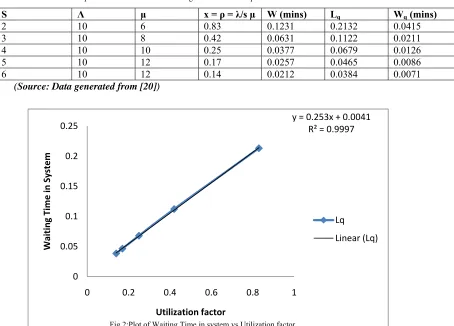
Table 4: Numerical representation of the Nonlinear Regression Model outputs.

S Λ µ x = ρ = λ/s µ W (mins) Lq Wq (mins)

2 10 6 0.83 0.1231 0.2132 0.0415

3 10 8 0.42 0.0631 0.1122 0.0211

4 10 10 0.25 0.0377 0.0679 0.0126

5 10 12 0.17 0.0257 0.0465 0.0086

6 10 12 0.14 0.0212 0.0384 0.0071

y = 0.253x + 0.0041 R² = 0.9997

0 0.05 0.1 0.15 0.2 0.25

0 0.2 0.4 0.6 0.8 1

Waiting

Time

in

System

Utilization factor

Fig 2:Plot of Waiting Time in system vs.Utilization factor

Lq

(8)

y = 0.253x + 0.0041 R² = 0.9997

0 0.05 0.1 0.15 0.2 0.25

0 0.2 0.4 0.6 0.8 1

Waiting

Time

in

Queue

Fig 3:Plot of Waiting Time in Queue vs.Utilization factor

Lq

Linear (Lq)

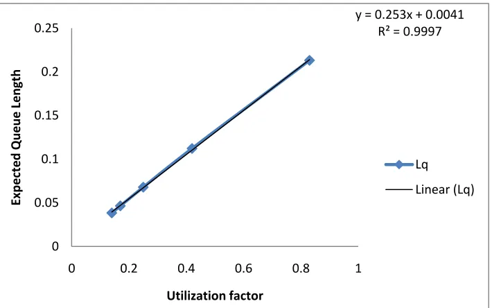
y = 0.253x + 0.0041 R² = 0.9997

0 0.05 0.1 0.15 0.2 0.25

0 0.2 0.4 0.6 0.8 1

Exp

ected

Queue

Length

Fig 4:Plot of Expected Queue Length vs.Utilization factor

Lq

(9)

Table 5: Computation of Error Analysis for waiting time in system

i. si λi μi Ρ W St=(W– W′₎2 _{Sr= (W-a0(1–e}a₁x₎₎2 1 2 10 6 0.83 0.1231 0.0047500 0.0000000019 2 3 10 8 0.42 0.0631 0.0000792 0.0000000013 3 4 10 10 0.25 0.0377 0.0002720 0.00000000067 4 5 10 12 0.17 0.0257 0.0008120 0.00000000019 5 6 10 12 0.14 0.0212 0.0010900 0.000000000027

0.2710 0.0070022 0.0000000041

The standard error is given by the expression:



1 

/



_

_

m

n

S

r

x

y (12) Hence, the standard error for the waiting time in system becomes:

Sy/x = 0.000037

Also, the coefficient of determination is given by the expression:

(13)

R2 ₌₁

This gives a Correlation coefficient of 1. Hence, the degree of correlation is 100%.

Table 6: Computation of Error Analysis for expected queue length

i. si λi μi ρ Lq St=(Lq- L′_q)2 _{Sr=(Lq-a0(1–e}-a1x₎₎2

1 2 10 6 0.83 0.2132 0.0138 0.00000000134

2 3 10 8 0.42 0.1122 0.000274 0.00000000115 3 4 10 10 0.25 0.0679 0.000770 0.00000000182 4 5 10 12 0.17 0.0465 0.002415 0.00000000000408 5 6 10 12 0.14 0.0384 0.003276 0.00000000000818

0.4782 0.0205 0.00000000432

From (12) the standard error for the expected queue length becomes: Sy/x = 0.000038

(10)

R2 ₌₁

This gives a Correlation coefficient of 1. Hence, the degree of correlation is 100%

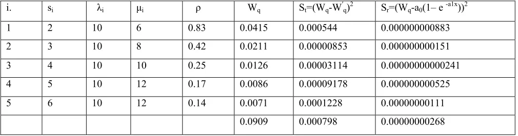
Table 7: Computation of Error Analysis for waiting time in queue

i. si λi μi ρ Wq St=(Wq-W′_q)2 _{Sr=(Wq-a0(1– e}-a1x₎₎2 1 2 10 6 0.83 0.0415 0.000544 0.000000000883 2 3 10 8 0.42 0.0211 0.00000853 0.000000000151 3 4 10 10 0.25 0.0126 0.00003114 0.00000000000241 4 5 10 12 0.17 0.0086 0.00009178 0.000000000525 5 6 10 12 0.14 0.0071 0.0001228 0.00000000111

0.0909 0.000798 0.00000000268

The standard error for the expected queue length is computed as: Sy/x = 0.0000299

The coefficient of determination is computed as:

R2 ₌₁

This gives a Correlation coefficient of 1. Hence, the degree of correlation is 100%

4. Discussion of Results

From figures 2, 3 and 4, the following were obtained:

 The Coefficient of determination, R2 value equals 1.  The Correlation coefficient also gives 1.

 The Degree of Correlation is 100%.

This result indicates that 100% of the original uncertainty has been explained by the model. Since the Degree of Correlation is 100%, the Nonlinear Regression Model output therefore supports the conclusion that the exponential equation represents an excellent fit in evaluating queuing problems.

One major importance of these models is that they are easily understood and more convenient for organizations to assess.

5. Conclusions

(11)

Furthermore, new mathematical models (Expected Queue Length, Waiting Time in Queue, and Waiting Time in the System) were created using the non linear regression approach which is validated using the Microsoft Excel. These models are more convenient for management to assess because they are easy to understand.

Finally, the most important aspect of the models created in this work is that it shows the management of any organization that despite the limited number of staff they have, they can distribute the available staff among the units effectively and efficiently.

6. References

[1] Brockmeyer, E., Halstrom, H. L. and Jensen, A. (1960). The Life and Works of A. K. Erlang, Acta Polytechnica Scandinavica, Applied

Math.and Comp. Machinery Series No. 6, Copenhagen.

[2] Molina, E. C. (1927). “Application of the theory of probability to telephone trunking problems”, Bell System Tech. J. 6, 461-494 [3] Gaver, D. P. Jr. (1968). “Diffusion approximations and models for certain congestion problems”, J. Appl. Prob. 5, 607-623. [4] Pollaczek, F. (1934). “Uber das Warteproblem”, Math. Zeitschrift, 38, 492-537.

[5] Pollaczek, F. (1965). “Concerning an analytical method for the treatment of queueing problems”, Proc. Symp. Congestion Theory (Eds. W. L.

Smith and W. E. Wilkinson), Univ. of North Carolina, Chapel Hill, 1-42.

[6] Syski, R. (1960). Introduction to Congestion Theory in Telephone Systems, Oliver and Boyd, London. [7] Saaty, T. L. (1961). Elements of Queueing Theory and Applications, Mc-Graw Hill Book Co., New York. [8] Bhat, U. N. (1969). “Sixty years of queueing theory”, Management Sci., 15 B, 280-294.

[9] Bailey, N. T. J. (1954). “A continuous time treatment of a simple queue using generating functions”, J. Roy. Statist. Soc. B, 16, 288-291.

[10] Ledermann, W. and Reuter, G. E. (1956). “Spectral theory for the differential equations of simple birth and death processes,” Phil. Trans. Roy.Soc., London A246, 321-369.

[11] Lindley, D. V. (1952). “The theory of queues with a single server”, Proc.Comb. Phil. Soc. 48, 277-289.

[12] Prabhu, N. U. and Bhat, U. N. (1963). “Some first passage problems and their application to queues”, Sankhya, Series A25, 281-292.

[13] Tak´acs, L. (1967). Combinatorial Methods in the Theory of Stochastic Processes, John Wiley & Sons, New York.

[14] Newel, G. F. (1968). “Queues with time dependent arrival rates I - III”, J.Appl. Prob. 5, 436-451, 579-606. [15] Newel, G. F. (1971). Applications of Queueing Theory (Ch. 6), Chapman and Hall, London.

[16] Kulkarni, V. G. and Liang, H. M. (1997). “Retrial queues revisited”, Frontiers in Queueing (Ed. J. H. Dshalalow), CRC Press, New York, Ch. 2, 19-34.

[17] Hillier, F. S. (1963). “Economic models for industrial waiting line problems”, Management Sci. 10, 119-130.

[18] Hillier F. S and Lieberman G.J, (2001),“Introduction to Operations Research”, McGraw – Hill,7th_Edition. [19] Heyman, D. P. (1968). “Optimal operating policies for M/G/1 queueing systems”, Operations Res.16, 362-382.

[20] Mgbemena, C.E. (2010), “Modelling of the Queueing System for Improved Customer Service in Nigerian Banks”, M.Eng Thesis, Nnamdi Azikiwe University, Awka, Nigeria.