https://doi.org/10.5194/cp-15-1251-2019 © Author(s) 2019. This work is distributed under the Creative Commons Attribution 4.0 License.
Last Millennium Reanalysis with an expanded proxy database
and seasonal proxy modeling
Robert Tardif1, Gregory J. Hakim1, Walter A. Perkins1, Kaleb A. Horlick2, Michael P. Erb3, Julien Emile-Geay4, David M. Anderson5, Eric J. Steig6,1, and David Noone2
1Department of Atmospheric Sciences, University of Washington, Seattle, WA, USA
2College of Earth, Ocean, and Atmospheric Sciences, Oregon State University, Corvallis, OR, USA
3School of Earth and Sustainability, Northern Arizona University, Flagstaff, AZ, USA
4Department of Earth Sciences, University of Southern California, Los Angeles, CA, USA
5Retired, NOAA Paleoclimatology Program, Boulder, CO, USA
6Department of Earth and Space Sciences, University of Washington, Seattle, WA, USA
Correspondence:Robert Tardif ([email protected])
Received: 7 September 2018 – Discussion started: 18 September 2018 Revised: 28 May 2019 – Accepted: 4 June 2019 – Published: 5 July 2019
Abstract.The Last Millennium Reanalysis (LMR) utilizes an ensemble methodology to assimilate paleoclimate data for the production of annually resolved climate field reconstruc-tions of the Common Era. Two key elements are the focus of this work: the set of assimilated proxy records and the forward models that map climate variables to proxy mea-surements. Results based on an updated proxy database and seasonal regression-based forward models are compared to the LMR prototype, which was based on a smaller set of proxy records and simpler proxy models formulated as uni-variate linear regressions against annual temperature. Val-idation against various instrumental-era gridded analyses shows that the new reconstructions of surface air temper-ature and 500 hPa geopotential height are significantly im-proved (from 10 % to more than 100 %), while improvements in reconstruction of the Palmer Drought Severity Index are more modest. Additional experiments designed to isolate the sources of improvement reveal the importance of the updated proxy records, including coral records for improving tropical reconstructions, and tree-ring density records for tempera-ture reconstructions, particularly in high northern latitudes. Proxy forward models that account for seasonal responses, and dependence on both temperature and moisture for tree-ring width, also contribute to improvements in reconstructed thermodynamic and hydroclimate variables in midlatitudes. The variability of temperature at multidecadal to centennial scales is also shown to be sensitive to the set of assimilated
proxies, especially to the inclusion of primarily moisture-sensitive tree-ring-width records.
1 Introduction
production of annually resolved reconstructions of the Com-mon Era. Hakim et al. (2016) describe a prototype configu-ration of the LMR and show results in good agreement with previous reconstructions of Northern Hemisphere mean near-surface air temperature. Detailed comparisons with several gridded instrumental temperature data products revealed sig-nificant skill over tropical regions but less skillful reconstruc-tions over Northern Hemisphere continental areas, where a large proportion of proxy data are located.
As with any data assimilation system, two of three im-portant components impacting the quality of the resulting analyses are the set of assimilated observations (here, proxy records) and the forward models that map variables from climate model output to proxy measurements (“proxy sys-tem models”; hereafter, PSMs). The third component is the model providing the prior state, although it is not the fo-cus of this work. Hakim et al. (2016) assimilated proxy records from the first compilation of the PAGES 2k Consor-tium (PAGES 2k ConsorConsor-tium, 2013) and modeled the prox-ies through univariate linear regressions calibrated against annually averaged instrumental temperature data. Here, we examine the impact on LMR reconstructions of improve-ments to these two key components: (1) an updated and ex-panded proxy database, primarily composed of records from PAGES 2k Consortium (2017), and assessment of the addi-tional records described in Anderson et al. (2019); (2) more realistic PSMs in which seasonality and, for tree-ring-width proxies, temperature and moisture sensitivity are taken into account. Motivation for expanding the proxy database de-rives from evidence that climate reconstructions are gener-ally sensitive to the set of proxy records used as input (e.g., Wang et al., 2015), while the introduction of more sophisti-cated PSMs is motivated in part by the fact that comprehen-sive reconstructions of temperature and hydroclimate vari-ables depend on properly treating temperature-sensitive and moisture-sensitive tree-ring proxies (e.g., Steiger and Smer-don, 2017).
The focus of improvements in PSMs here is on regression-based (i.e., statistical) forward models, in contrast to recent efforts focusing on process-based PSMs (see, e.g., Breiten-moser et al., 2014; Dee et al., 2016; Acevedo et al., 2017). Our objective is to establish baseline skill of PDA reconstruc-tions using statistical PSMs to serve as a benchmark for eval-uating possible improvements associated with process-based PSMs (e.g., Dee et al., 2016). Here, we develop a hierar-chy of statistical PSMs to identify aspects that contribute in-creased skill to reconstructed temperature and hydroclimate states compared to the prototype LMR.
The remainder of the paper is organized as follows. Sec-tion 2 outlines the LMR PDA-based framework and de-scribes the proxy database and PSMs. Reconstructions based on this configuration are presented in Sect. 3, with compar-isons to the prototype described in Hakim et al. (2016). Sec-tion 4 explores the contribuSec-tions to improvements in the new reconstructions. A concluding summary is given in Sect. 5.
2 Methods
Paleoclimate data assimilation has three main components: proxy records, providing an indirect record of past climatic conditions; climate models, providing prior estimates of the climate; and proxy system models, providing the connection between the model prior and the proxy values. The method for each component is now described.
2.1 Data assimilation framework
LMR employs ensemble data assimilation (DA) to blend in-formation from proxies and climate model data. DA is per-formed using a variant of the ensemble Kalman filter, which for our application appears to perform well compared to al-ternative PDA methods such as particle filters (Liu et al., 2017). The update equation is given by
xa=xb+K[y−ye]. (1)
Here,xb is the prior state vector, which contains the cli-mate variables to be reconstructed, averaged over an appro-priate timescale (here, annual), andxais the posterior state vector (i.e., the reanalysis, or reconstruction). The state vec-tor may include scalars, such as climate indices, and/or grid-point data for spatial fields. Vectorycontains the assimilated proxy data (i.e., observations), andyeis a vector containing estimates of the proxies derived from the prior by
ye=H(xb), (2)
whereHis the forward model mapping the priorxbto proxy space (i.e., the PSM; see Sect. 2.4). The innovation, [y–ye], is the new information from the proxies not already contained in the prior. This new information is weighted against the prior through the Kalman gain matrix:
K=BHTHBHT+R−1, (3)
whereBis the prior covariance matrix,Ris the error covari-ance matrix for the proxy data, andHis the linearization of
the singlekth proxyyk, are obtained from
xa=xb+
wloc◦cov(xb, ye,k) var(ye,k)+Rk
(yk−ye,k) (4a)
x0a=x0b− "
1+
s
Rk var(ye,k)+Rk
#−1
wloc◦cov(xb, ye,k) var(ye,k)+Rk
(y0e,k), (4b)
whereye,kis the prior estimate of the proxy from Eq. (2),Rk is the diagonal element ofRcorresponding to proxyyk, and cov() and var() represent the covariance and variance func-tions, respectively. The ensemble of updated states is then recovered by combining the posterior ensemble mean and perturbations:
xa=xa+x0a. (5)
Covariance localization, given by a Schur product denoted by ◦ in Eq. (4b) (i.e., element-wise multiplication), is a distance-weighted filterwlocon the prior covariance matrix (see, e.g., Hamill et al., 2001). Sections 4.2 and S5 in the Supplement provide more details on localization.
We also use an “appended state vector” approach that avoids the need to recompute Eq. (2) after each proxy is as-similated. The yeproxy estimates from each record are ap-pended to the state vectorxb:
xb=
x1 .. . xN
ye1
.. .
yeP
, (6)
where thex1. . .xN elements contain the ensemble grid-point data from model variables included in the state (e.g., tem-perature, precipitation), with N the sum of the number of variables multiplied by the number of grid points, and the ye1. . .yeP are the ensemble proxy estimates for each of theP proxy records considered. Each of thex1. . .xN andye1. . .yeP elements are of dimensions 1×Nens, whereNensis the speci-fied size of the ensemble. Hence,xbis a matrix of dimension (N+P)×Nens. With such an appended state, theyeelements in Eq. (6) are updated through Eq. (4b) as any other state variables, eliminating the need to re-evaluateyewith Eq. (2) once the state has been updated. This simplification is par-ticularly attractive in the context of LMR updates discussed herein as it enables a straightforward implementation of sea-sonal PSMs (i.e., forward models more accurately represent-ing the seasonal responses of individual proxy records) as discussed in Sect. 2.4. In our implementation for the recon-struction of annually averaged states, the data assimilation procedure follows this general algorithm.
1. The proxy estimates (ye) are precalculated using Eq. (2) with either annually or seasonally averaged model data as input (i.e., thexbin Eq. 2).
2. A sample ensemble of annually averaged model states is randomly drawn from a pre-existing simulation to form the main part of the prior state vector (i.e., thex1. . .xN elements in Eq. 6).
3. The precalculatedye1. . .yeP proxy estimates are added on to form the appended state as shown in Eq. (6). This appended state becomes thexbin Eq. (1), which is de-composed into an ensemble mean (xb) and perturba-tions about the mean (x0b) as shown in Eq. (4b).
4. Proxies forming theyvector are then serially processed, with the updated state, including the proxy estimates, obtained from Eq. (4b). The reanalysis is completed for 1 year once all proxies have been assimilated.
We note here that with a configuration involving seasonal PSMs without the use of an appended state, the vectorxbhas to include states with sufficient temporal resolution to allow the calculation of the updated seasonaly1e. . .yeP proxy esti-mates. In this scenario, an additional step to the ones listed above is required, involving Eq. (2) using the appropriate sea-sonally averaged updated states as input. With proxies char-acterized by a wide range of seasonal responses, this require-ment would impose anxbcomposed of monthly data which would greatly increase the computational cost of the reanal-ysis. Reanalysis results would also likely be adversely af-fected by the larger noise level characterizing data at shorter (i.e., monthly) timescales through its impact on ensemble es-timates of prior covariances (see, e.g., Tardif et al., 2015).
Figure 1.Locations(a, c)and temporal(b, d)distributions of proxy records available for assimilation (proxies for which linear PSMs calibrated with GISTEMP version 4 are available). Panels(a, b)are used in the prototype version,(c, d)LMR proxy database updated to PAGES 2k Consortium (2017) proxies.
on an annual basis. This scenario is further supported by the PDA results of Matsikaris et al. (2015), who show similar performance is achieved with online and offline approaches. From a cost–benefit perspective, the high cost of running en-sembles of comprehensive global climate model simulations does not appear justified. However, ongoing research sug-gests cost-effective online PDA may be achieved by using simplified climate models (Perkins and Hakim, 2017).
2.2 Climate proxies
Our proxy database is updated to the latest PAGES 2k col-lection (PAGES 2k Consortium, 2017, hereafter PAGES2k-2017). This data set represents the community standard in global proxy observations covering the Common Era (CE) and serves as the core source of proxy information used in our updated reanalysis. PAGES2k-2017 proxies were screened to retain temperature-sensitive records, extensively quality controlled, and described by more metadata com-pared to previous collections. The additional records
as-sembled by Anderson et al. (2019)1, consisting in large part of the tree-ring-width records from Breitenmoser et al. (2014) (hereafter B14), are considered as a potential en-hancement to proxy information used in our paleoreanalyses (see Sect. 4.3).
As in the LMR prototype (Hakim et al., 2016, hereafter H16), only records with sub-annual to annual resolutions are considered; sub-annual records are averaged to annual. Fig-ure 1 compares the PAGES 2k Consortium (2013) (hereafter 2013) data set used in H16 and the PAGES2k-2017 update. Only records for which a PSM can be estab-lished are shown in Fig. 1, defined by proxy records with at least 25 years of (non-contiguous) overlap with calibration data (see Sect. 2.4). Compared to the proxies assimilated in H16, PAGES2k-2017 data provide enhanced spatial coverage in the tropics with additional coralδ18O and Sr/Ca records.
1An exception is the use of the Palmyra coral record from Cobb
Additional tree-ring wood-density records from Europe and western North America are also included. The temporal dis-tribution of the total number of records remains similar, ex-cept for significant increases in the number of tree-ring-width and coral proxies during 1800–2000 CE and tree-ring wood-density records during 1500–2000 CE.
2.3 Climate model prior information
For all reconstruction experiments reported in this paper, the prior state vector is formed with data from the Cou-pled Model Intercomparison Project phase 5 (CMIP5) (Tay-lor et al., 2012) Last Millennium simulation from the Com-munity Climate System Model version 4 (CCSM4) cou-pled atmosphere–ocean–sea-ice model. The simulation cov-ers years 850 to 1850 CE and includes incoming solar vari-ability and variable greenhouse gases, as well as stratospheric aerosols from volcanic eruptions known to have occurred during the simulation period (see Landrum et al., 2013). The same “offline” DA methodology as in H16 is used, where the prior ensemble is a random sample of model states, with the same sample used for all years of the reconstruction. The sampled states are deviations (i.e., anomalies) from the temporal mean taken over the entire length of the simula-tion. Therefore, the prior ensemble mean does not contain time-specific information about climate events (e.g., a vol-canic eruption) or trends characterizing specific periods (e.g., 20th century warming). Consequently, all trends and tem-poral structure in reconstructed fields result from informa-tion provided by the proxies. Finally, the spatial resoluinforma-tion of prior state variables is reduced from 0.95◦×1.25◦of the Last Millennium simulation to a 4.3◦×5.7◦Gaussian grid as in H16.
All reconstruction experiments are composed of 51 Monte Carlo assimilation realizations, each using a different ran-domly chosen 100-member ensemble and 75 % of available proxy records for assimilation. This Monte Carlo sampling over subsets of prior states and proxy records is designed to incorporate uncertainties in covariance estimates derived from model states and uncertainties associated with proxy er-ror estimates. Moreover, we have found that averaging over ensembles from Monte Carlo realizations leads to more accu-rate results. This is likely the result of averaging over random errors introduced into the reanalysis from a few randomly chosen proxy records with underestimated observation er-rors. Little sensitivity to the use of 75 % of the proxies for each realization has been found (not shown), while 100 mem-bers have been chosen to maintain consistency with H16. In the following, climate reanalyses are taken as the mean over the 100-member DA ensembles and 51 Monte Carlo realiza-tions (i.e., a 5100-member “grand ensemble”).
2.4 Proxy modeling
A critical component of PDA is the mapping of prior climate state variables (e.g., temperature, precipitation from a cli-mate model) to the assimilated proxies (e.g., tree-ring width). This is expressed mathematically by Eq. (2), Sect. 2.1, where the operatorH(i.e., the forward model) ideally represents the complete set of processes associated with proxy values, i.e., a comprehensive physically based PSM. This remains a major challenge as the information archive is often com-plex, involving physical, biological and chemical processes (Evans et al., 2013). Despite recent progress in the develop-ment and use of process-based PSMs (e.g., Dee et al., 2015, 2016; Goosse, 2016; Steiger et al., 2017; Acevedo et al., 2017), the focus here is on statistical PSMs, which offer dis-tinct advantages: (1) ease of implementation and flexibility with respect to forward modeling of multiple proxies, regard-less of archive types, measurements, units, etc.; (2) observa-tion error statistics for each assimilated record are well de-fined from the regression (see below); and (3) regressions are formulated on the basis of deviations from the mean over a reference period (e.g., 1951–1980) of the driving climate variable(s), therefore avoiding issues with absolute calibra-tion where climate model bias is problematic, particularly for PSMs having threshold transitions (see, e.g., Dee et al., 2016). Statistical PSMs also have distinct disadvantages: (1) PSMs cannot be calibrated without sufficient overlap with calibration data (a threshold of at least 25 overlapping data is imposed); (2) the accuracy of the models depends on the limitations of the calibration data sets (e.g., less reliable anal-ysis over the Southern Ocean and over high-latitude conti-nental areas due to a lack of observations); (3) possible lack of stationarity of the derived relationships established with instrumental-era data; and (4) lack of representation of non-linear and/or multivariate influences when PSMs are formu-lated as linear univariate models. Despite these limitations, statistical PSMs provide advantageous capabilities within the context of the LMR and moreover define a baseline to mea-sure future progress with the development of process-based PSMs.
Here, univariate and bivariate statistical PSMs are consid-ered:
yk =β0k +β1kX10+k, (7)
and
yk =β0k +β1kX10+β2kX20+k, (8)
zero mean and varianceσ2. The overbar in Eqs. (7) and (8) denotes time averages over annual periods, as in H16, or over appropriate seasonal intervals for the seasonal PSMs. Cal-ibration data concurrent with available proxy observations are taken at the grid point nearest the proxy location and the appropriate least-squares solution determines regression pa-rameters (β0, β1, β2, σ). In this version of LMR, PSM config-uration is the same for each proxy category (e.g., univariate for all coralδ18O, bivariate for all tree-ring-width records).
With the framework described above, the regression-based approach measures the diagonal elements in matrix R through the variance of regression residuals, i.e., Rk=
σ2. This is a key parameter in PDA as it determines the extent to which the information provided by the proxy is weighted against prior information in the resulting reanal-ysis. This method provides a sound basis through which as-similated proxy records influence the reanalysis depending on the strength of their relationship to the dependent climate variables. For example, a record with a poor fit to calibration data will be characterized by larger residuals, hence larger observation error variance, and less weight in the reanalysis relative to a record that has a stronger correlation with cli-mate variables. We note that modestly different results are obtained with different observational calibration data sets (see H16).
The calibration data sets used in this study are the NASA Goddard Institute for Space Studies (GISS) Surface Tem-perature Analysis (GISTEMP) (Hansen et al., 2010) ver-sion 4 for temperature and the gridded precipitation data set from the Global Precipitation Climatology Centre (GPCC) (Schneider et al., 2014) version 6 as the source of monthly information on moisture input over land surfaces. The use of precipitation instead of the more traditional Palmer Drought Severity Index (PDSI) to account for moisture is described in more detail in Sect. S4 of the Supplement.
2.4.1 Seasonality
Here, we take advantage of the availability of expert infor-mation about the seasonal response to temperature for each proxy record included in the PAGES2k-2017 metadata. This information is not available in PAGES2k-2013, hence lead-ing to the use of PSMs calibrated on annual averages for all records in H16. Seasonality information is provided for each record as a numerical representation of a sequence of con-secutive months (e.g., JJA as [6,7,8]). Seasonal PSMs are de-rived by using this sequence as the averaging period defining X10andX20in Eqs. (7) and (8).
Precise information on proxy seasonality is, however, not available for all records in the updated LMR proxy database. The proxies from Anderson et al. (2019), for example, have not been subjected to extensive community-wide screening and vetting as with the PAGES2k-2017 proxies. In particular, seasonality information for the large number of additional tree-ring records from B14 has been encoded using a
sim-ple latitudinal dependence which does not attempt to repre-sent possible record-by-record diversity (see Anderson et al., 2019). This lack of expert-informed seasonality motivates an objective alternative to the metadata seasonality informa-tion for calibrating tree-ring-width (TRW) forward models. We consider several potential seasonal periods, perform a gression over each possible season and identify the linear re-lationship providing the best fit to proxy values, as defined by the maximum value of the adjustedR2, a goodness-of-fit measure defined as (Goldberger, 1964, p. 217)
Radj2 =1−
"
1−R2 (N−1) N−M−1
#
. (9)
Here,R2 is the variance explained by the linear model,N is the sample size, and M is the number of predictors in the model. The adjustedR2 penalizes complexity (i.e., the number of predictors) of the model in such a way that val-ues characterizing a more complex model will increase only if the additional predictors improve the fit more than would be expected by chance. Test periods considered include, in addition to the seasonal response in the proxy metadata (if available), the calendar year, boreal summer (JJA) and bo-real winter (DJF), and extended spring and fall growing sea-sons (MAMJJA, JJASON for NH trees; SONDJF, DJFMAM for SH trees) to account for ecosystem-dependent variations in tree growth shifted toward the earlier or later parts of the warm season (see, e.g., Sano et al., 2009; D’Arrigo et al., 2005). With this test set of seasonal responses, the dominant sensitivity of some TRW chronologies to winter tempera-ture (D’Arrigo et al., 2012) is included, as well as the win-ter and spring precipitation sensitivities characwin-terizing some tree species (see, e.g., Stahle et al., 2009; Touchan et al., 2003). The latter point is germane to the calibration of sea-sonal TRW models using precipitation as a predictor (see the next section).
2.4.2 Tree-ring-width sensitivity to temperature and moisture
Proxy number is strongly dominated by TRW records in the LMR proxy database, particularly with the addition of chronologies from B14. Furthermore, these records have not been screened on temperature, which opens the opportunity to measure moisture sensitivity through the regression frame-work. The addition of an explanatory variable increases the potential for overfitting, and our framework is designed to measure that using the 25 % of proxies withheld from assim-ilation, for which we can measure reconstruction errors and compare results with proxies that were assimilated (see dis-cussion of proxy verification results in Sect. 3).
pre-cipitation. For each TRW record, distinct regressions with either variable are established and the model providing the best fit to proxy data is selected. Following a common prac-tice in dendroclimatology, this approach determines whether the record is predominantly temperature or moisture limited (see, e.g., St. George, 2014). Similar univariate “temperature or moisture” models (abbreviated as “TorM” hereafter) are successfully used in Steiger et al. (2018). The second method consists of simultaneously factoring both temperature and moisture sensitivities through the bivariate relationship ex-pressed in Eq. (8).
Seasonal univariate TorM and bivariate TRW models are considered, with distinct sets of models calibrated using proxy seasonality either from the proxy metadata or objec-tively derived during calibration. This selection has impor-tant implications for the representation of the proxy seasonal response to moisture in particular. For the proxy metadata, seasonality for moisture is assumed to be identical to temper-ature, as this is the only information available, whereas the objective approach allows for independent encoding of sea-sonal responses to temperature and moisture. For TorM mod-els, the objective seasonality for univariate moisture models is independent of temperature as it is determined solely from the fit to precipitation data. For bivariate PSMs, all possible combinations of seasonal responses specified independently for temperature and moisture are considered, and the com-bination providing the best fit is selected. With such flexi-bility, TRW models with objectively derived seasonality are expected to provide a more realistic representation of the sig-nificant variability in seasonal responses to moisture charac-terizing TRW records (see, e.g., St. George et al., 2010). We note that this approach is similar to the methodology used to calibrate the VS-Lite model (Tolwinski-Ward et al., 2011), in that grid cell temperature and precipitation data are used to determine site-specific growth seasons and seasonally de-pendent temperature and moisture growth parameters.
An examination of PSM characteristics, summarized here, with more detail provided in Appendix A, confirms that prox-ies are represented more accurately by seasonal models, par-ticularly for tree-ring wood-density and width records (see Table A1). Moreover, more accurate fits to TRW data are obtained when proxy seasonal responses are determined ob-jectively during model calibration. Finally, the addition of moisture input as a climate driver in TRW modeling proves most beneficial when implemented in bivariate models (see Table A2). These findings serve as the basis for defining a PDA configuration used for the reconstruction described in the next section.
3 The updated reanalysis
We present a comparison between the updated reanalysis de-scribed by the method in the previous section with the LMR
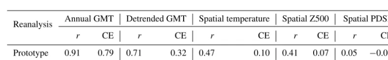
prototype described in H162. Specifically, the updated re-analysis consists of proxy records from the PAGES2k-2017 collection, using objectively derived seasonal PSMs, with a bivariate formulation for all TRW proxies and univariate for all other proxy types. Covariance localization is applied with a 25 000 km cut-off radius (see Sect. 4.2 for more details). In the next section, we identify the sources of improvement that contribute to the increase in skill of the updated recon-struction. Results are evaluated against various 20th century instrumental data and reanalyses, as well as verification per-formed in proxy space, using the Pearson correlation coef-ficient and the coefcoef-ficient of efficiency (CE) (Nash and Sut-cliffe, 1970). These skill scores are complementary since cor-relation measures signal timing, while CE, based on mean square error with climatology as a reference, is sensitive to bias and errors in signal amplitude.
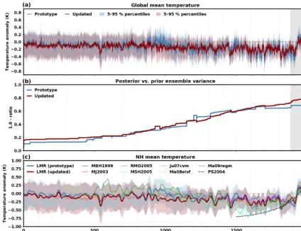
Figure 2a shows a comparison of reconstructed global-mean temperature (GMT) between the prototype and updated reanalyses over the entire Common Era. Similar features are observed in the ensemble mean from both reanalyses, namely the cooling trend over most of the Common Era, followed by the industrial-era warming. Superimposed on these main trends, significant multidecadal to multicentennial variability characterizes both reanalyses, including a cool period prior to the industrial warming, consistent with the Little Ice Age (LIA). Differences also exist between the reanalyses, most noticeably the absence in the updated LMR of the relatively warm period during 870–1000 CE, representing the Medieval Climate Anomaly (MCA). Also, warmer conditions prevail in the prototype during the second half of the 15th century, while cooler conditions occur during the early part of the instrumental period in the prototype compared to the up-dated reanalysis. We note, however, that verification against instrumental-era temperature analyses (discussed later in the section) provides evidence that the prototype reanalysis is too cold during that period.
Ensembles provide access to useful diagnostics regarding reconstruction uncertainty. It can be shown mathematically that the assimilation of observations monotonically reduces the variance of the posterior ensemble compared to the prior. The ratio of ensemble variance of the posterior (reanalysis) to the prior is a measure of the information provided by the assimilated proxies. Figure 2b shows the temporal evolution of 1−var[xa]/var[xb], so that a value of 0 indicates no in-fluence from proxies, and 1 implies that all error has been removed. In the early part of the Common Era, when few proxy data are available, variance decreases of only 10 %– 15 % occur in the prototype compared to 15 %–20 % for the updated reanalysis. The influence of proxies gradually in-creases after 450 CE, at similar rates in both reanalyses. The
2We use the experiment included in Fig. 12 of H16, with PSMs
Figure 2.Comparison of the LMR global-mean 2 m air temperature (GMT)(a)grand ensemble mean (solid lines) and 5th—95th percentile range (shading) from the prototype (blue) and updated (red) reanalyses over the Common Era and(b)1 minus the mean (across Monte Carlo realizations) ratio of the posterior and prior GMT ensemble variance.(c)Comparison of the LMR Northern Hemisphere 2 m air temperature grand ensemble mean (solid lines) and 5th–95th percentile range (shading) from the prototype and updated reanalyses with reconstructions from other authors; MBH1999: Mann et al. (1999), MJ2003: Mann and Jones (2003), RMO2005: Rutherford et al. (2005), MSH2005: Moberg et al. (2005), Ju07cvm: Juckes et al. (2007), Ma08eivf: Mann et al. (2008), Ma09regm: Mann et al. (2009), PS2004: Pollack and Smerdon (2004). All series in panel(c)represent anomalies (Kelvin, K) from the 1900–1980 mean and have been smoothed with a 30-year low-pass Butterworth filter. The light gray shading in panels(a)and(b)indicates the verification period discussed in Fig. 3.
reductions in variance are roughly similar in both reanaly-ses until 1700 CE, corresponding to the period with a signifi-cantly larger number of proxies in the updated database (see Fig. 1). The largest reduction, 68 % in the prototype com-pared to 78 % in the updated reanalysis, is found during the 20th century when the most proxies are available, which un-derscores the importance of the expanded proxy database in LMR.
To gain further perspective on our results, we compare the reconstructed Northern Hemisphere average 2 m air tempera-ture from the prototype and updated reanalyses with other re-constructions quoted in the Intergovernmental Panel on Cli-mate Change Fourth and Fifth Assessment Reports (IPCC AR4 and AR5) (Fig. 2c). Here, we restrict the comparison to reconstructions covering the entire hemisphere and having a temporal coverage extending to at least 1980. A 30-year low-pass Butterworth filter is applied on all results to highlight
re-cent PAGES 2k Consortium (2017) proxy data. A distinctly warmer medieval period is not a prominent feature of the new collection, as indicated by the global temperature compos-ites presented in PAGES 2k Consortium (2017). Second, the colder temperatures in the updated reanalysis during the late 15th and early 16th centuries are in better agreement with the majority of reconstructions in other studies, with respect to both the magnitude and trend of temperature anomalies. The LMR prototype appears as a warm outlier for this 100-year period. In contrast, the prototype LMR appears as a cold outlier during the latter part of the 19th and early 20th cen-turies. During that period, the updated reanalysis is in bet-ter agreement with results from other authors, in particular with the borehole temperature reconstruction by Pollack and Smerdon (2004).
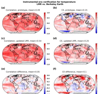
GMT verification results of the LMR ensemble mean against various instrumental temperature products are shown in Fig. 3a and b for the prototype and updated reanalyses, respectively. Noticeably higher verification scores character-ize the updated LMR, including a 9 % increase in CE rela-tive to the average of observation-based temperature analyses (“consensus”), and an increase in CE in the verification of the detrended GMT (over 1880–2000 CE) from 0.32 in the pro-totype to 0.59 in the updated reanalysis (see Table 1). Spatial verification is provided by comparing the LMR gridded 2 m air temperature field against the Berkeley Earth instrumental-era tempinstrumental-erature analysis (Rohde et al., 2013) (Fig. 4). Berke-ley Earth is chosen as the verification reference, as it is not used to calibrate the PSMs, and provides the most complete spatial coverage compared to other instrumental products. The updated temperature reconstruction is largely improved compared to the prototype over large areas, including the tropical Pacific, northern Atlantic, western North America, northern Europe, central Asia and Oceania, and over portions of the Pacific sector of the Southern Ocean. The improve-ment is reflected in both correlation and CE scores, indicating improved timing and amplitude in reconstructed temperature variability. Exceptions are found over parts of the southern Atlantic and Indian oceans, although the decrease in skill is generally more modest compared to the magnitude of im-provements elsewhere.
Next, we verify a climate variable away from the sur-face, the 500 hPa geopotential height field, against the corre-sponding field from NOAA’s 20th century reanalysis (20CR-v2; Compo et al., 2011) (Fig. 5). Once again, we find the largest improvements over extratropical continental loca-tions and over the Arctic. We note similar improvements are found over the Northern Hemisphere midlatitudes when verified against the ERA-20C reanalysis (Poli et al., 2016) (not shown); however, over the Northern Hemisphere, high-latitude verification against ERA-20C is worse, which under-scores significant differences between 20th century reanaly-ses in these data-sparse regions.
Table 1 summarizes the verification results discussed above through globally averaged verification scores. The
ta-ble also includes verification results of reconstructed PDSI, not discussed above. A more detailed analysis for this vari-able is reserved for Sect. 4.3, where the role of additional proxy records is discussed. Improvements in the updated re-analyses are evident for all reconstructed variables, particu-larly with respect to the CE score, which is sensitive to bias and amplitude in interannual variability. These skill improve-ments suggest significant positive impact from the updated tropical coral proxies and tree-ring proxies at higher lati-tudes. Furthermore, we anticipate that generalizing PSMs to accounting for seasonality and moisture sensitivity for TRW proxies also contributes to the improvements.
We consider now an independent evaluation of the recon-structions in proxy space using proxies withheld from as-similation. Proxy time series estimated (forward modeled) from the posterior (i.e., the reconstructions) are compared to the actual proxy observations and various skill metrics are evaluated. Verification of proxy estimates obtained from the uninformed climate model prior serves as a reference for comparison. Specifically, we use the change in CE between the posterior proxy estimates and estimates obtained from the prior,1CE=(CEposterior−CEprior). Values are compiled from all proxy records withheld from assimilation, and the following summary scores are considered: the fraction of all proxy records which are characterized by a positive 1CE (i.e., proxy records more accurately represented in the poste-rior than in the pposte-rior) and the median of the1CE distribution compiled over all proxy time series. These provide global summary measures of how reanalyses skill differs from the prior. An additional discriminating factor on the quality of the reanalysis is “ensemble calibration”, as defined by Mur-phy (1988):
ECR=
" 1 N−1
N X
n=1
(vn−xn)2 #
" 1 N−1
N X
n=1
(σx,n2 +σv,n2 ) #−1
, (10)
pe-Figure 3.Comparison of LMR global-mean 2 m air temperature (GMT)(a)prototype and(b)updated reanalyses, against instrumental-era analyses (GISTEMP: NASA GISS surface tempinstrumental-erature (Hansen et al., 2010); HadCRUT4: Hadley Center/Climate Research Unit at the University of East Anglia temperature data set version 4 (Morice et al., 2012); BE: Berkeley Earth surface temperature (Rohde et al., 2013); NOAAGlobalTemp:NOAA merged land–ocean surface temperature version 3.5.4 (Smith et al., 2008); 20CR-v2: NOAA 20th century reanalysis version 2 (Compo et al., 2011); ERA-20C: ECMWF reanalysis of the 20th century (Poli et al., 2016); consensus: average of all but LMR). The gray bands show the LMR 5th–95th percentile range. Verification correlation (r) and coefficient of efficiency (CE) values are shown at the bottom of each panel for the original and detrended time series.
Table 1.Summary of instrumental-era verification results for the prototype and updated reanalyses. Verification scores shown arerand CE for the annual GMT and detrended GMT verified against the consensus of instrumental-era analyses, the global mean of grid pointr and CE characterizing the spatially reconstructed temperature, 500 hPa geopotential height (Z500) and Palmer Drought Severity Index (PDSI). LMR spatial temperature is verified against the Berkeley Earth analysis (Rohde et al., 2013), Z500 is verified against the 20CR-v2 reanalysis (Compo et al., 2011), and PDSI is verified against the Dai (2011) analysis.
Reanalysis Annual GMT Detrended GMT Spatial temperature Spatial Z500 Spatial PDSI
r CE r CE r CE r CE r CE
Prototype 0.91 0.79 0.71 0.32 0.47 0.10 0.41 0.07 0.05 −0.03 Updated 0.93 0.86 0.77 0.59 0.52 0.22 0.45 0.18 0.09 0.00
riods of the Common Era. Significantly reduced skill char-acterizes the earliest period of the Common Era, followed by a continuous increase over time in all verification metrics considered, for both LMR reanalyses. We also note that re-analysis ensembles are generally well calibrated throughout the Common Era, indicating that respective uncertainties re-main consistent with mean errors (i.e., reliable ensembles). Although verification data are not identical between proto-type and updated reanalyses, we also note that the increase in skill is more pronounced in the updated reanalysis, partic-ularly from 1000 CE onward. These results provide further evidence of a more skillful updated LMR. In the following section, we systematically evaluate improvements from vari-ous sources.
4 Sources of improvement
In this section, we identify the sources of reanalysis improve-ment. Results from multiple reconstruction experiments are presented, designed to quantify the impact of PSM formula-tion, the role of covariance localization and the assimilation of additional proxies.
4.1 Proxy system models
The different PSM configurations described in Sect. 2.4 are used in a series of reconstruction experiments using PAGES2k-2017 proxies exclusively. We note that these records have well-defined seasonal metadata.
deter-Figure 4.Verification of LMR 2 m air temperature against the Berkeley Earth instrumental-era analysis over the 1880–2000 period. Shown are time series correlation(a, c, e)and CE (b, d, f) for(a, b)the prototype and(c, d)the updated reanalysis. Differences in correlations and CE between the two experiments are shown in panels(e)and(f), respectively. Gray shading indicates regions with insufficient valid data for meaningful verification statistics.
Table 2.Verification of LMR prototype and updated reanalyses against independent (withheld from assimilation) proxies. Skill scores shown are the median of distributions forr, the fraction of proxy records characterized by a positive1CE (%+CE) and the median of the1CE distribution, where1CE is the difference in the CE between the posterior (reanalysis) and the prior. The median of the ensemble calibration ratio (ECR) distribution is also shown. Statistics are compiled over 51 Monte Carlo realizations and cover different time periods, including the 1880–2000 PSM calibration period.
Verification period (years of Common Era) Prototype Updated reanalysis
r %+CE 1CE ECR r %+CE 1CE ECR
1–499 0.00 56.0 0.00 0.78 0.03 55.9 0.00 0.96
500–999 0.08 62.1 0.01 1.00 0.13 65.3 0.02 1.00
1000–1499 0.11 63.0 0.01 1.10 0.16 67.3 0.05 1.06
1500–1879 0.14 64.1 0.02 1.06 0.28 72.7 0.10 1.02
1880–2000 0.23 72.6 0.03 0.97 0.40 82.7 0.13 0.89
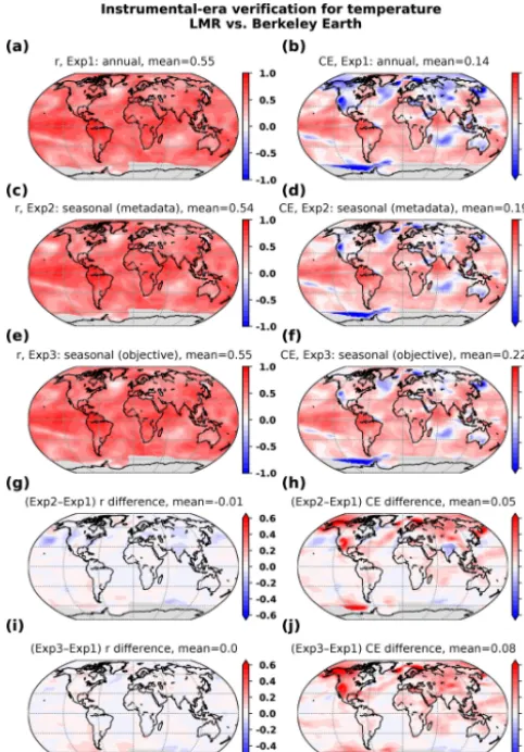
mined seasonality. Performance is again measured by cor-relation and CE scores with verification against the Berke-ley Earth analysis. Relative to reconstructions with annual-mean PSMs (Fig. 6a and b), the reconstructions with sea-sonal PSMs (Fig. 6c–f) show improvements in both mea-sures over nearly the entire globe (Fig. 6g–j). Results show a larger improvement for CE (Fig. 6h and j) compared to
Figure 5.As in Fig. 4 except for the verification of LMR 500 hPa geopotential height anomalies against the 20CR-v2 reanalysis.
Antarctic Peninsula (see Fig. 6h). Comparing the differences of correlations and CE in Fig. 6i and j to those shown in Fig. 6g and h reveals that PSMs with objectively derived sea-sonality contribute positively to skill for the aforementioned regions, especially where tree-ring-width records are most abundant (e.g., North America and Asia).
We turn now to the impact of moisture on seasonal TRW PSMs on the reconstructions. Since objectively defined sea-sonality performs best (i.e., Fig. 6e and f), reconstructions generated with univariate PSMs are used as the reference for measuring skill improvements for modeling TRW records as univariate in either temperature or moisture (abbreviated as “TorM”) (Fig. 7c and d) and for bivariate “temperature and moisture” PSMs (Fig. 7e and f). Improvement over univari-ate PSMs is apparent for the bivariunivari-ate approach compared with the univariate “TorM” approach (cf. Fig. 7g, h with i, j, respectively). In the bivariate approach, regions such as west-ern North America and central Asia, where most of the TRW records are found, improve the most in CE, but also over Australia, likely in response to the improved modeling of TRW records in New Zealand and Tasmania. Improvements are also noticeable, through teleconnections with proxy loca-tions in the central Atlantic and southern Indian oceans, and over the eastern North Pacific Ocean. A decrease in skill is
present over the midlatitude Pacific Ocean, but this is smaller in magnitude compared with skill enhancements elsewhere.
Verification of GMT for reconstructions using seasonal PSMs (Table 3) yields a similar interpretation to the spa-tial verification results. Compared to the consensus of instrumental-era products, we find that the 20th century trend in GMT is overestimated with the PAGES2k-2017 proxy data set if univariate PSMs are used. This is particularly the case with annual PSMs. Better agreement is obtained when sea-sonal bivariate PSMs are used to model TRW proxies. The representation of GMT interannual variability as measured by verification of the detrended GMT is also improved with seasonal PSMs, particularly for the CE metric. Similar to spatial verification results, PSMs with objectively derived seasonality and bivariate TRW modeling have GMT recon-structions with consistently higher skill scores.
Table 3.Summary of instrumental-era verification results for reconstruction experiments performed with various PSM configurations. Veri-fication scores shown are the trend over the 20th century (in K/100 years),rand CE for the annual GMT and detrended GMT verified against the consensus of instrumental-era analyses. The GMT trend in the consensus of instrumental-era analyses is 0.56 K/100 years.
PSM configuration GMT trend Annual GMT Detrended GMT
r CE r CE
Prototype 0.61 0.91 0.79 0.71 0.32
Univariate – temperature (annual) 0.85 0.93 0.61 0.74 0.39 Univariate – temperature (seasonal meta.) 0.72 0.93 0.77 0.73 0.43 Univariate – temperature (seasonal obj.) 0.72 0.93 0.80 0.75 0.51 Univariate – temperature or moisture (TRW) (seasonal meta.) 0.71 0.92 0.78 0.72 0.44 Univariate – temperature or moisture (TRW) (seasonal obj.) 0.74 0.93 0.77 0.74 0.48 Bivariate – temperature and moisture (TRW) (seasonal meta.) 0.62 0.93 0.84 0.76 0.50 Bivariate – temperature and moisture (TRW) (seasonal obj.) 0.60 0.93 0.86 0.77 0.54
Results from these experiments, described in Sect. S3 in the Supplement, confirm the main results and conclusions drawn here on the superiority of seasonal PSMs relative to those cal-ibrated with annual averages and the use of bivariate models for TRW proxies.
We now examine results from an evaluation performed in proxy space using proxies withheld from assimilation as in Sect. 3. Results for both the PSM calibration and pre-calibration periods are shown in Table 4. Differences among the various experiments suggest the superiority of the sea-sonal (with objective seasea-sonality) PSMs as skill scores con-sistently rank among the highest among all experiments for both calibration and pre-calibration periods. The recon-struction using univariate annual PSMs shows the weakest verification statistics, confirming the verification based on instrumental-era analyses. Finally, use of bivariate seasonal PSMs for TRW records is also suggested from proxy valida-tion results, as larger correlavalida-tions and1CE are obtained with this configuration.
4.2 Covariance localization
One approach to managing sampling error in ensemble data assimilation is through spatial covariance localization. Local-ization is applied to minimize the adverse impact of spurious covariances at large distances from a proxy location, which results from sample error in finite ensembles (Hamill et al., 2001). If localization is not applied, spurious covariances al-low proxies to affect remote locations, which adversely af-fects the quality of the analysis. On the other hand, too-short localization length scales reduce the useful information that can be derived from the proxies. Therefore, a balance is sought between minimizing sampling noise versus retaining useful proxy information.
We use the Gaspari–Cohn (Gaspari and Cohn, 1999) fifth-order polynomial with a specified cut-off radius for the local-ization function (wlocin Eq. 4b). See Sect. S5 for information on the characteristics ofwloc. A series of reconstructions is performed with a wide range of localization length scales.
As with previous experiments, 51 Monte Carlo realizations are carried out, each with 100 ensemble members assimilat-ing 75 % of proxy records. Results from the instrumental-era verification scores previously described are summarized in Table 5. We observe that the GMT trend is underestimated and verification scores are significantly reduced when “too-small” localization radii are used, indicating the information on temperature provided by some proxy records is not prop-erly incorporated in the reanalysis. In contrast, the trend is overestimated and verification scores are generally reduced without covariance localization. This is particularly the case for the CE score for the detrended GMT, sensitive to the am-plitude in interannual variability. This skill measure is max-imized for localization radii within the 15 000 to 25 000 km range. A localization radius at the upper end of this range (25 000 km) is preferable, as results from the other verifica-tion scores suggest that a skillful reconstrucverifica-tion is obtained with this covariance localization configuration. See Fig. S4 for an example where the 25 000 km localization function is applied to a proxy record located in California, United States. We note that the optimal localization radius depends on a number of factors, such as ensemble size, the observation network and observation error characteristics.
4.3 Proxy data sets
Table 4.Verification of LMR reconstructions against independent (withheld from assimilation) proxies for experiments using various PSM configurations. Skill scores shown are the median of distributions forr, the fraction of proxy records characterized by a positive1CE (%+CE) and the median of the1CE distribution. Statistics are compiled over 51 Monte Carlo realizations for two distinct periods: 1880– 2000 (PSM calibration period) and 0–1879 (pre-calibration period).
PSM configuration 1880–2000 1–1879
r %+CE 1CE r %+CE 1CE
Univariate - temperature (annual) 0.28 75.2 0.05 0.17 66.0 0.03 Univariate – temperature (seasonal meta.) 0.32 78.7 0.06 0.21 69.6 0.04 Univariate – temperature (seasonal obj.) 0.34 80.6 0.09 0.21 69.4 0.06 Univariate – temperature or moisture (TRW) (seasonal meta.) 0.30 76.1 0.06 0.19 67.7 0.04 Univariate – temperature or moisture (TRW) (seasonal obj.) 0.33 77.6 0.08 0.19 66.3 0.04 Bivariate – temperature and moisture (TRW) (seasonal meta.) 0.32 77.9 0.07 0.20 68.1 0.04 Bivariate – temperature and moisture (TRW) (seasonal obj.) 0.36 78.9 0.11 0.22 66.0 0.06
Table 5.The 20th century trend of GMT,rand CE, for the annual and detrended GMTs, as well as the global mean of the spatial (i.e., grid point)rand CE of reconstructed temperature verified against the consensus of instrumental-era analyses for reconstruction experiments performed with covariance localization using various localization cut-off radii (LR). Verification statistics for an experiment without covari-ance localization are also shown for comparison. Results from the prototype are shown for reference. The GMT trend in the consensus of instrumental-era analyses is 0.56 K/100 years.
LR LR LR LR LR LR No Prototype
5000 km 10 000 km 15 000 km 25 000 km 35 000 km 45 000 km localization (no localization)
Trend (K/100 years) 0.17 0.31 0.40 0.49 0.51 0.56 0.60 0.61
Annual GMTr 0.92 0.93 0.93 0.93 0.93 0.93 0.93 0.91
Annual GMT CE 0.46 0.71 0.82 0.86 0.87 0.87 0.86 0.79
Detrended GMTr 0.74 0.77 0.77 0.77 0.77 0.76 0.77 0.71
Detrended GMT CE 0.35 0.53 0.59 0.59 0.58 0.56 0.54 0.32
Mean spatialr 0.36 0.46 0.50 0.52 0.52 0.53 0.53 0.47
Mean spatial CE 0.11 0.17 0.19 0.22 0.21 0.21 0.20 0.10
provide additional records in the tropics (23 coral records) and an enhanced number of ice core records concentrated over Greenland and the eastern Canadian Arctic (37 records) and Antarctica (26 records in West Antarctica and Dron-ning Maud Land). A few lower-latitude ice core records (six records) are also added in the Peruvian Andes and Tibetan Plateau, along with two higher-latitude lake core records. From a temporal perspective, the addition of the B14 tree-ring-width records contributes a notable number of addi-tional proxies back to 1000 CE, more than double the number of records available for assimilation from 1500 CE onward, up to a 4-fold increase during the 19th and 20th centuries.
In order to measure the impact with the best configura-tion, the reconstruction experiments reported in this section are carried out using seasonal PSMs with objectively derived seasonality for all records, with a bivariate formulation on temperature and precipitation for all TRW proxies and uni-variate on temperature for all other proxies. The baseline re-construction uses the PAGES2k-2017 proxies (as in Sect. 3), which we compare to results first obtained with the addition of the B14 TRW records and finally with the further addition of the coral, ice and lake core records from A19 (i.e., the full
proxy database). Other trial reconstructions performed with the vastly expanded proxy network, not reported here, show that a well-calibrated GMT ensemble is obtained with a co-variance localization cut-off radius of 25 000 km. Next, we compare reconstruction results from this configuration to the baseline reanalysis.
Differences in correlation and CE associated with the ad-dition of the B14 collection over the PAGES2k-2017 prox-ies show skill improvements in temperature reconstructions over the continental United States and Mexico, Europe and the southern edge of the Tibetan Plateau (see Fig. 9g and h). Through the influence of significant spatial covariances with the added records, assimilation of the additional TRW records also leads to improved temperature skill over remote areas of the midlatitude Pacific and northern Atlantic oceans. The addition of records described in A19 has minimal addi-tional impact overall, with the exception of modest increases in correlation and CE over Greenland (see Fig. 9i and j).
Figure 6.Verification of LMR temperature anomalies against the Berkeley Earth instrumental-era analysis, for experiments using PAGES2k-2017 proxies and univariate PSMs, with contrasting sea-sonalities. Shown are time seriesrand CE for(a, b)experiment 1: annual, (c, d)experiment 2: seasonality from the proxy metadata and(e, f)experiment 3: objectively derived seasonality. Differences in skill metrics are also shown(g, h)between experiments 2 and 1, and(i, j)between experiments 3 and 1.
calibrated on precipitation and not on PDSI as in Steiger et al. (2018). A comparison of the reconstructed PDSI between the prototype3, the updated reanalysis of Sect. 3 and a recon-struction carried out with the B14 TRW records and the addi-tional coral, ice and lake core records (i.e., the full database) is shown in Fig. 10. The PDSI is slightly improved in the up-dated reanalysis compared to the prototype (Fig. 10g and h). Enhanced skill is noticeable over western North America and over eastern Europe and Asia to a lesser degree. Decreased skill is found over the central plains of North America and along a narrow band along the Siberian Taiga. The impact of adding the Anderson et al. (2019) records is mostly found
3The LMR prototype configuration has been used to reconstruct
PDSI, a variable not included in H16, for the purpose of this com-parison.
Figure 7.As in Fig. 6 but comparing experiments performed us-ing PAGES2k-2017 proxies with different PSM configurations for tree-ring-width proxies.(a, b)Experiment 1: univariate on temper-ature for all proxies,(c, d)experiment 2: univariate with respect to temperature or moisture for TRWs and(e, f)experiment 3: bivari-ate on temperature and moisture for tree-ring widths. Differences in skill metrics are shown(g, h)between experiments 2 and 1, and (i, j)between experiments 3 and 1. All reconstructions are based on objectively derived seasonal PSMs.
over the eastern part of the United States and over western Europe (Fig. 10i and j). Finally, we note that this impact is due entirely to the B14 TRW records, as the additional coral, ice and lake core records from A19 do not significantly af-fect the PDSI reconstruction skill (from results of additional reconstruction experiments carried out to isolate this impact; not shown).
com-Figure 8.Locations(a)and temporal distributions(b)of the additional proxies from Anderson et al. (2019) considered for assimilation, including the tree-ring chronologies from Breitenmoser et al. (2014). As in Fig. 1, only records available for assimilation (proxies for which regression-based PSMs can be calibrated) are shown.
Table 6.As in Table 4 but statistics compiled for tree-ring wood-density (MXD) proxies only, and for experiments using the PAGES2k-2017 proxies only, PAGES2k-PAGES2k-2017 with the addition of all proxies from A19 (all proxies) and PAGES2k-PAGES2k-2017 plus only a subset of A19 records obtained after removing all but 188 TRW records from B14 (B14 subset). See text for selection details. Skill scores are the median ofrdistributions, the fraction of proxy records characterized by a positive1CE (%+CE) and the median of1CE distributions. Statistics are compiled over the 51 Monte Carlo realizations for the following periods: 1880–2000 (PSM calibration period) and 1600–1879 (pre-calibration period with a significant number of MXD records and covering a significant portion of the Little Ice Age).
PSM configuration 1880–2000 1600–1879
r %+CE 1CE r %+CE 1CE
PAGES2k-2017 0.62 93.2 0.37 0.58 91.4 0.39 All proxies 0.43 88.0 0.18 0.46 95.4 0.26 B14 subset 0.56 92.5 0.30 0.53 93.8 0.34
paring spectra from both experiments (Fig. 11c). This loss of variability in the reconstruction using all proxies occurs at nearly all scales, underlining an adverse impact from assim-ilating B14 tree-ring-width proxies.
We now turn to verification in proxy space, which is the only source available prior to the instrumental period. Proxy estimates from reanalyses (estimated using the appropriate PSM) are compared directly to proxy observations. Here, re-analysis skill is assessed using independent (the 25 % with-held from assimilation) proxies. We further restrict our anal-ysis to verification against tree-ring wood-density proxies, as they are among the most reliable recorders of tempera-ture in our database, as evidenced by the generally better fits to calibration temperature data obtained when calibrat-ing the univariate PSMs. Also, these proxies provide good temporal coverage of the latter portion of the LIA into the industrial period, as shown in Fig. 1. The results, presented in Table 6, show distinctly larger skill scores for the experi-ment using PAGES2k-2017 proxies only compared to when all proxies are assimilated. Improved skill is observed for
Figure 9.As in Fig. 6 but comparing experiments performed with different proxy networks:(a)rand(b)CE for experiment 1: PAGES 2k Consortium (2017) proxies only,(c, d)experiment 2: with the ad-dition of tree-ring chronologies from Breitenmoser et al. (2014) and (e, f)experiment 3: with all proxies in the updated LMR database. The differences in correlation and CE between experiments 2 and 1 are shown in panels(g, h), respectively, and between experiments 3 and 2 in panels(i, j). Notice the latter is different from Fig. 6, where differences between experiments 3 and 1 are shown.
selection of these records requires further careful attention and could serve as the basis for future efforts.
5 Concluding summary
A paleoclimate reanalysis of the Common Era has been de-veloped using an updated data assimilation framework. Re-sults show significant improvement over the prototype Last Millennium Reanalysis presented in Hakim et al. (2016). An updated proxy database and implementation of PSMs with improved realism are shown to be key contributors to the en-hanced reanalysis. The main upgrade to the proxy database consists of a change from the community standard of PAGES 2k Consortium (2013) to the more recent PAGES 2k Consor-tium (2017) data set, while the records described in Anderson
Figure 10.Similar to Fig. 9 but comparing PDSI reconstructions against the Dai (2011) analysis for experiments performed with dif-ferent proxy networks:(a)correlation and(b)CE for experiment 1: prototype reanalysis from H16, experiment 2: PAGES 2k Consor-tium (2017) proxies,(e, f)experiment 3: with further the addition of tree-ring chronologies from Breitenmoser et al. (2014) and the coral, ice and lake core records from Anderson et al. (2019) (i.e., the full proxy database). The differences in correlation and CE be-tween experiments 2 and 1 are shown in panels(g, h), respectively, and between experiments 3 and 2 in panels(i, j).
et al. (2019) remain available for possible future enhance-ments to the proxy information used in the reanalysis. More-over, new methods to map state variables to observations ex-tend the prototype’s linear univariate models calibrated on annual-mean temperature in two key aspects: accounting for seasonal dependencies of individual proxy records and the modeling of tree-ring-width proxies using temperature and moisture as predictors. The encoding of proxy seasonality in-formation within PSMs has also been refined by objectively determining the characteristic seasonal response of individ-ual records and by decoupling the seasonality for temperature and precipitation sensitivity for tree-ring width.
con-Figure 11.(a)Northern Hemisphere temperature (NHMT) grand ensemble mean (solid lines) and 5th—95th percentile range (shad-ing) from experiments performed with PAGES2k-2017 proxies (in blue) and with the addition of proxies from Anderson et al. (2019) (in red). (b) Spectra of NHMT grand ensemble mean from both experiments (solid lines), along with theχ295 % highest density regions (shading).
figurations have been compared to available instrumental-era observation-based analyses, revealing notable improve-ments not only in the reconstructed global-mean temperature in general but also in reconstructed spatial fields. More skill-ful tropical Pacific temperatures are obtained primarily due to the updated set of coral records in the PAGES 2k Con-sortium (2017) collection. Improved temperature reconstruc-tions over continental extratropical regions are the result of the newly implemented seasonal PSMs, combined with the forward modeling of tree-ring-width chronologies using a bi-variate temperature–moisture formulation. Improvements are reflected not only in temperature reconstructions but also in 500 hPa geopotential height and to some extent in hydrocli-mate variables such as the PDSI. Lastly, the introduction of the large collection of Breitenmoser et al. (2014) tree-ring-width chronologies, not screened for temperature sensitivity, appears to provide local skill enhancements in hydroclimate variables (e.g., PDSI over the eastern United States). How-ever, this is achieved at the expense of accuracy in the re-construction of important features of pre-industrial climate such as the colder temperatures during the Little Ice Age. However, the generally positive impact of a simple ad hoc screening of the Breitenmoser et al. (2014) suggests that fur-ther improvements may be possible with a careful selection of tree-ring chronologies.
Results presented here, based upon regression PSMs, may serve as a reference for future efforts designed to assess the value of more comprehensive process-based PSMs in paleoclimate data assimilation research. Finally, we note that the version of the PDA system described here cor-responds to the configuration used in the production re-lease of the NOAA Last Millennium Reanalysis, avail-able at https://atmos.washington.edu/~hakim/lmr/ (last ac-cess: 30 June 2019).
Code availability. The code used in the production of reanalyses is publicly available at https://github.com/modons/LMR (Hakim, 2019a)
Appendix A: Proxy system model characteristics
Features introduced in the updated LMR proxy modeling ca-pabilities include a representation of the seasonal response to climate drivers characterizing individual proxy records (i.e., proxy seasonality), as well as PSMs that include precipita-tion and temperature as driving variables for modeling TRW records.
The first approach is to use univariate PSMs calibrated against temperature data, with proxy seasonality either de-fined from the available proxy metadata or derived objec-tively using the method described in Sect. 2.4.1. PSM perfor-mance is compared using the Bayesian information criterion (BIC), defined as (Schwarz, 1978)
BIC= −2 ln(Lˆ)+kln(n), (A1)
whereLˆ is the maximized value of the likelihood function of the model, n is the sample size andk is the number of estimated parameters in the model. We note that the second term in Eq. (A1) represents a penalty for models with a larger number of explanatory variables, i.e., a more complex model. This feature is particularly useful when comparing univariate and bivariate models. Here, we use the difference in BIC val-ues between two models, 1BIC=(BICM−BICref), to de-termine the relative accuracy of model Mover a reference. The model with the lowest BIC is preferred (i.e., a better fit to the data); hence, a negative1BIC indicates the superior-ity of the test model over its reference. Here, the seasonal PSMs are tested against the univariate PSMs calibrated with annually averaged temperatures as the reference. Significant evidence of the superiority of the test model over its refer-ence is obtained when1BIC<−2.0.
Table A1 presents a summary of1BIC results for records in each proxy category considered in LMR. The advantage of seasonal PSMs is particularly significant for tree-ring wood-density chronologies, a proxy known for its strong seasonal response (Briffa et al., 2004). Seasonal PSMs also provide improved fits to tree-ring-width data, although to a lesser extent compared to density records. As indicated by the larger negative 1BIC values, models based on objectively derived seasonal responses lead to more accurate descrip-tions of proxy data compared to those calibrated using meta-data seasonality, even for tree-ring chronologies within the community-curated PAGES2k-2017 data set. These results suggest that the objectively derived seasonality information is noticeably different than in the metadata, particularly for tree-ring records in the Breitenmoser et al. (2014) (i.e., B14) data set, but also for those in PAGES 2k Consortium (2017) (i.e., PAGES2k-2017). More details on this aspect are pro-vided in the Supplement. The use of objectively defined sea-sonality improves upon the simple latitude-dependent rela-tionship described in Anderson et al. (2019), more consis-tent with records from the PAGES2k-2017 data set. Apart from lake sediment records, which are also more accurately modeled with seasonal PSMs, Table A1 shows that PSMs for
other proxy types are not as sensitive to seasonality. In fact, the majority of the (tropical) coral records included in the current database have metadata seasonality defined as annual already, as do the high-latitude ice core records. Note that some of these records originate from the collection described by Anderson et al. (2019), where seasonal metadata informa-tion is generally not available. As a result, these records are assumed to be annual.
In addition to seasonal models, other improvements in-volve the development of PSMs that add precipitation as an input variable for the modeling of TRW proxies as outlined in Sect. 2.4.2. One approach consists of selecting the uni-variate models, either calibrated on temperature or moisture input, which best describe the proxy data. This “tempera-ture or mois“tempera-ture” selection (abbreviated as “TorM”) is per-formed on individual TRW records, and the resulting pro-portion of TRW proxies identified as temperature-sensitive is 56.4 % versus 43.6 % for moisture when metadata season-ality information is considered. This is compared to 36.8 % temperature-sensitive versus 63.2 % moisture-sensitive trees when seasonal responses are determined objectively. The latter option, leading to a larger proportion of moisture-sensitive records, is in better agreement with a comparable characterization performed by Steiger et al. (2018) on a sim-ilar set of TRW records.
Table A1.Mean differences in Bayesian information criterion (1BIC) corresponding to PSMs for records within the proxy categories considered in LMR, between models calibrated using proxy seasonal responses from the metadata or derived objectively during calibration, with respect to the reference of annual seasonality. Calibration data set: GISTEMP v4.
Proxy types Number of records Seasonal (metadata) Seasonal (objective)
Tree-ring width (PAGES2k-2017) 347 −1.34 −4.84
Tree-ring width (Breitenmoser et al., 2014) 2156 −1.72 −5.24
Tree-ring wood density 59 −23.28 NA
Coralδ18O 75 +0.02 NA
Coral Sr/Ca 30 −0.01 NA
Coral rates 11 +0.03 NA
Ice coreδ18O 89 +0.02 NA
Ice coreδD 12 0.00 NA
Ice core accumulation 3 0.00 NA
Ice core melt 1 0.00 NA
Lake core varve 7 −0.52 NA
Lake core misc. 2 −2.32 NA
Bivalveδ18O 1 0.00 NA
Tree-ringδ18O 1 +11.81 NA
NA: not available.
Table A2.Mean differences in Bayesian information criterion (1BIC) for tree-ring-width univariate “temperature or moisture” and bivariate PSMs, calibrated using metadata seasonality or derived objectively during calibration, against their respective univariate temperature-only PSMs as reference. Calibration data sets: GISTEMP v4 and GPCC v6.
PSM formulation Seasonal (metadata) Seasonal (objective) PAGES 2k trees Breitenmoser trees PAGES 2k trees Breitenmoser trees
Univariate – temperature or moisture −0.86 −1.41 −2.59 −6.65