Optimizing HPC Applications with Intel Cluster Tools

(1)

Shelve in Software Engineering/Software Development User level: Intermediate–Advanced

Optimizing HPC Applications

with Intel

®

Cluster Tools

Optimizing HPC Applications with Intel®_{Cluster Tools}_{takes the reader on a tour} of the fast-growing area of high performance computing and the optimization of hybrid programs. These programs typically combine distributed memory and shared memory programming models and use the Message Passing Interface (MPI) and OpenMP for multi-threading to achieve the ultimate goal of high performance at low power consumption on enterprise-class workstations and compute clusters.

The book focuses on optimization for clusters consisting of the Intel®_Xeon

processor, but the optimization methodologies also apply to the Intel®_{Xeon Phi™}

coprocessor and heterogeneous clusters mixing both architectures. Besides the tutorial and reference content, the authors address and refute many myths and misconceptions surrounding the topic. The text is augmented and enriched by descriptions of real-life situations.

What You’ll Learn:

• Practical, hands-on examples show how to make clusters and workstations based on Intel®_{Xeon processors and Intel}®_{Xeon Phi™ coprocessors}

“sing” in Linux environments

• How to master the synergy of Intel®_{Parallel Studio XE 2015 Cluster Edition,}

which includes Intel®_{Composer XE, Intel}®_{MPI Library, Intel}®_{Trace Analyzer}

and Collector, Intel®_{VTune™ Amplifier XE, and many other useful tools} • How to achieve immediate and tangible optimization results while refining

your understanding of software design principles

Supalov

Semin

Klemm

Dahnken

(2)

For your convenience Apress has placed some of the front

matter material after the index. Please use the Bookmarks

and Contents at a Glance links to access them.

(3)

Contents at a Glance

About the Authors ��

xiii

About the Technical Reviewers ��

xv

Acknowledgments ��

xvii

Foreword ��

xix

Introduction ��

xxi

Chapter 1: No Time to Read This Book?

■

��

1 Chapter 2: Overview of Platform Architectures

■

��

11 Chapter 3: Top-Down Software Optimization

■

��

39 Chapter 4: Addressing System Bottlenecks

■

��

55 Chapter 5: Addressing Application Bottlenecks:

■

Distributed Memory ��

87 Chapter 6: Addressing Application Bottlenecks:

■

Shared Memory ��

173 Chapter 7: Addressing Application Bottlenecks:

■

Microarchitecture ��

201 Chapter 8: Application Design Considerations

■

��

247

(4)

Introduction

Let’s optimize some programs. We have been doing this for years, and we still love doing it. One day we thought, Why not share this fun with the world? And just a year later, here we are.

Oh, you just need your program to run faster NOW? We understand. Go to Chapter 1 and get quick tuning advice. You can return later to see how the magic works.

Are you a student? Perfect. This book may help you pass that “Software Optimization 101” exam. Talking seriously about programming is a cool party trick, too. Try it.

Are you a professional? Good. You have hit the one-stop-shopping point for Intel’s proven top-down optimization methodology and Intel Cluster Studio that includes Message Passing Interface* (MPI), OpenMP, math libraries, compilers, and more.

Or are you just curious? Read on. You will learn how high-performance computing makes your life safer, your car faster, and your day brighter.

And, by the way: You will find all you need to carry on, including free trial software, code snippets, checklists, expert advice, fellow readers, and more at

www.apress.com/source-code.

HPC: The Ever-Moving Frontier

High-performance computing, or simply HPC, is mostly concerned with

floating-point operations per second, or FLOPS. The more FLOPS you get, the better. For convenience, FLOPS on large HPC systems are typically counted by the quadrillions (tera, or 10 to the power of 12) and by the quintillions (peta, or 10 to the power of 15)—hence, TeraFLOPS and PetaFLOPS. Performance of stand-alone computers is currently hovering at around 1 to 2 TeraFLOPS, which is three orders of magnitude below PetaFLOPS. In other words, you need around a thousand modern computers to get to the PetaFLOPS level for the whole system. This will not stay this way forever, for HPC is an ever-moving frontier: ExaFLOPS are three orders of magnitude above PetaFLOPS, and whole countries are setting their sights on reaching this level of performance now.

We have come a long way since the days when computing started in earnest. Back then [sigh!], just before WWII, computing speed was indicated by the two hours necessary to crack the daily key settings of the Enigma encryption machine. It is indicative that already then the computations were being done in parallel: each of the several “bombs”1

united six reconstructed Enigma machines and reportedly relieved a hundred human operators from boring and repetitive tasks.

(5)

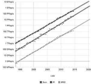
Computing has progressed a lot since those heady days. There is hardly a better illustration of this than the famous TOP500 list.2_{Twice a year, the teams running the}

most powerful non-classified computers on earth report their performance. This data is then collated and published in time for two major annual trade shows: the International Supercomputing Conference (ISC), typically held in Europe in June; and the Supercomputing (SC), traditionally held in the United States in November.

Figure 1 shows how certain aspects of this list have changed over time.

(6)

There are several observations we can make looking at this graph:3

1� Performance available in every represented category is growing exponentially (hence, linear graphs in this logarithmic representation).

2� Only part of this growth comes from the incessant improvement of processor technology, as represented, for example, by Moore’s Law.4_{The other part is coming from}

putting many machines together to form still larger machines. 3� An extrapolation made on the data obtained so far predicts

that an ExaFLOPS machine is likely to appear by 2018. Very soon (around 2016) there may be PetaFLOPS machines at personal disposal.

So, it’s time to learn how to optimize programs for these systems.

Why Optimize?

Optimization is probably the most profitable time investment an engineer can make, as far as programming is concerned. Indeed, a day spent optimizing a program that takes an hour to complete may decrease the program turn-around time by half. This means that after 48 runs, you will recover the time invested in optimization, and then move into the black.

Optimization is also a measure of software maturity. Donald Knuth famously said, “Premature optimization is the root of all evil,”5_{and he was right in some sense. We will}

deal with how far this goes when we get closer to the end of this book. In any case, no one should start optimizing what has not been proven to work correctly in the first place. And a correct program is still a very rare and very satisfying piece of art.

Yes, this is not a typo: art. Despite zillions of thick volumes that have been written and the conferences held on a daily basis, programming is still more art than science. Likewise, for the process of program optimization. It is somewhat akin to architecture: it must include flight of fantasy, forensic attention to detail, deep knowledge of underlying materials, and wide expertise in the prior art. Only this combination—and something else, something intangible and exciting, something we call “talent”—makes a good programmer in general and a good optimizer in particular.

Finally, optimization is fun. Some 25 years later, one of us still cherishes the memories of a day when he made a certain graphical program run 300 times faster than it used to. A screen update that had been taking half a minute in the morning became almost instantaneous by midnight. It felt almost like love.

The Top-down Optimization Method

(7)

The good news are, once you know what you want to achieve, the methodology is roughly the same. We will look into those details in Chapter 3. Briefly, you proceed in the top-down fashion from the higher levels of the problem under analysis (platform, distributed memory, shared memory, microarchitecture), iterate in a closed-loop manner until you exhaust optimization opportunities at each of these levels. Keep in mind that a problem fixed at one level may expose a problem somewhere else, so you may need to revisit those higher levels once more.

This approach crystallized quite a while ago. Its previous reincarnation was formulated by Intel application engineers working in Intel’s application solution centers in the 1990’s.6_{Our book builds on that solid foundation, certainly taking some things a tad}

further to account for the time passed.

Now, what happens when top-down optimization meets the closed-loop approach? Well, this is a happy marriage. Every single level of the top-down method can be handled by the closed-loop approach. Moreover, the top-down method itself can be enclosed in another, bigger closed loop where every iteration addresses the biggest remaining problem at any level where it has been detected. This way, you keep your priorities straight and helps you stay focused.

Intel Parallel Studio XE Cluster Edition

Let there be no mistake: the bulk of HPC is still made up by C and Fortran, MPI, OpenMP, Linux OS, and Intel Xeon processors. This is what we will focus on, with occasional excursions into several adjacent areas.

There are many good parallel programming packages around, some of them available for free, some sold commercially. However, to the best of our absolutely unbiased professional knowledge, for completeness none of them comes in anywhere close to Intel Parallel Studio XE Cluster Edition.7

Indeed, just look at what it has to offer—and for a very modest price that does not depend on the size of the machines you are going to use, or indeed on their number.

Intel Parallel Studio XE Cluster Edition

• 8_{compilers and libraries,}

including:

Intel Fortran Compiler

• 9

Intel C++ Compiler

• 10

Intel Cilk Plus

• 11

Intel Math Kernel Library (MKL)

• 12

Intel Integrated Performance Primitives (IPP)

• 13

Intel Threading Building Blocks (TBB)

• 14

Intel MPI Benchmarks (IMB)

• 15

Intel MPI Library

• 16

Intel Trace Analyzer and Collector

(8)

Intel VTune Amplifier XE

• 18

Intel Inspector XE

• 19

Intel Advisor XE

• 20

All these riches and beauty work on the Linux and Microsoft Windows OS, sometimes more; support all modern Intel platforms, including, of course, Intel Xeon processors and Intel Xeon Phi coprocessors; and come at a cumulative discount akin to the miracles of the Arabian 1001 Nights. Best of all, Intel runtime libraries come traditionally free of charge.

Certainly, there are good tools beyond Intel Parallel Studio XE Cluster Edition, both offered by Intel and available in the world at large. Whenever possible and sensible, we employ those tools in this book, highlighting their relative advantages and drawbacks compared to those described above. Some of these tools come as open source, some come with the operating system involved; some can be evaluated for free, while others may have to be purchased. While considering the alternative tools, we focus mostly on the open-source, free alternatives that are easy to get and simple to use.

The Chapters of this Book

This is what awaits you, chapter by chapter:

1� No Time to Read This Book? helps you out on the burning optimization assignment by providing several proven recipes out of an Intel application engineer’s magic toolbox.

2� Overview of Platform Architectures introduces common terminology, outlines performance features in modern processors and platforms, and shows you how to estimate peak performance for a particular target platform. 3� Top-down Software Optimization introduces the generic

top-down software optimization process flow and the closed-loop approach that will help you keep the challenge of multilevel optimization under secure control.

4� Addressing System Bottlenecks demonstrates how you can utilize Intel Cluster Studio XE and other tools to discover and remove system bottlenecks as limiting factors to the maximum achievable application performance. 5� Addressing Application Bottlenecks: Distributed Memory

shows how you can identify and remove distributed memory bottlenecks using Intel MPI Library, Intel Trace Analyzer and Collector, and other tools.

(9)

7� Addressing Application Bottlenecks: Microarchitecture

demonstrates how you can identify and remove microarchitecture bottlenecks using Intel VTune Amplifier XE and Intel

Composer XE, as well as other tools.

8� Application Design Considerations deals with the key tradeoffs guiding the design and optimization of applications. You will learn how to make your next program be fast from the start.

Most chapters are sufficiently self-contained to permit individual reading in any order. However, if you are interested in one particular optimization aspect, you may decide to go through those chapters that naturally cover that topic. Here is a recommended reading guide for several selected topics:

System optimization

• : Chapters 2, 3, and 4.

Distributed memory optimization

Shared memory optimization

Microarchitecture optimization

Use your judgment and common sense to find your way around. Good luck!

References

1. “Bomba_(cryptography),” [Online]. Available:

http://en.wikipedia.org/wiki/Bomba_(cryptography).

2. Top500.Org, “TOP500 Supercomputer Sites,” [Online]. Available: http://www.top500.org/.

3. Top500.Org, “Performance Development TOP500 Supercomputer Sites,” [Online]. Available: http://www.top500.org/statistics/ perfdevel/.

4. G. E. Moore, “Cramming More Components onto Integrated Circuits,” Electronics, p. 114–117, 19 April 1965.

5. “Knuth,” [Online]. Available: http://en.wikiquote.org/wiki/ Donald_Knuth.

6. Intel Corporation, “ASC Performance Methodology - Top-Down/ Closed Loop Approach,” 1999. [Online]. Available:

http://smartdata.usbid.com/datasheets/usbid/2001/2001-q1/ asc_methodology.pdf.

(10)

8. Intel Corporation, “Intel Composer XE,” [Online]. Available: http://software.intel.com/en-us/intel-composer-xe/.

9. Intel Corporation, “Intel Fortran Compiler,” [Online]. Available: http://software.intel.com/en-us/fortran-compilers.

10. Intel Corporation, “Intel C++ Compiler,” [Online]. Available: http://software.intel.com/en-us/c-compilers.

11. Intel Corporation, “Intel Cilk Plus,” [Online]. Available: http://software.intel.com/en-us/intel-cilk-plus.

12. Intel Corporation, “Intel Math Kernel Library,” [Online]. Available: http://software.intel.com/en-us/intel-mkl.

13. Intel Corporation, “Intel Performance Primitives,” [Online]. Available: http://software.intel.com/en-us/intel-ipp.

14. Intel Corporation, “Intel Threading Building Blocks,” [Online]. Available: http://software.intel.com/en-us/intel-tbb.

15. Intel Corporation, “Intel MPI Benchmarks,” [Online]. Available: http://software.intel.com/en-us/articles/intel-mpi-benchmarks/.

16. Intel Corporation, “Intel MPI Library,” [Online]. Available: http://software.intel.com/en-us/intel-mpi-library/.

17. Intel Corporation, “Intel Trace Analyzer and Collector,” [Online]. Available: http://software.intel.com/en-us/intel-trace-analyzer/.

18. Intel Corporation, “Intel VTune Amplifier XE,” [Online]. Available: http://software.intel.com/en-us/intel-vtune-amplifier-xe.

19. Intel Corporation, “Intel Inspector XE,” [Online]. Available: http://software.intel.com/en-us/intel-inspector-xe/.

(11)

No Time to Read This Book?

We know what it feels like to be under pressure. Try out a few quick and proven optimization stunts described below. They may provide a good enough performance gain right away.

There are several parameters that can be adjusted with relative ease. Here are the steps we follow when hard pressed:

Use Intel MPI Library

• 1_{and Intel Composer XE}2

Got more time? Tune Intel MPI:

•

Collect built-in statistics data •

Tune Intel MPI process placement and pinning •

Tune OpenMP thread pinning •

Got still more time? Tune Intel Composer XE:

•

Analyze optimization and vectorization reports •

Use interprocedural optimization •

Using Intel MPI Library

The Intel MPI Library delivers good out-of-the-box performance for bandwidth-bound applications. If your application belongs to this popular class, you should feel the difference immediately when switching over.

If your application has been built for Intel MPI compatible distributions like MPICH,3_MVAPICH2,4_{or IBM POE,}5_{and some others, there is no need to recompile the}

application. You can switch by dynamically linking the Intel MPI 5.0 libraries at runtime:

$ source /opt/intel/impi_latest/bin64/mpivars.sh $ mpirun -np 16 -ppn 2 xhpl

If you use another MPI and have access to the application source code, you can rebuild your application using Intel MPI compiler scripts:

Use

• mpicc (for C), mpicxx (for C++), and mpifc/mpif77/mpif90

(12)

Using Intel Composer XE

The invocation of the Intel Composer XE is largely compatible with the widely used GNU Compiler Collection (GCC). This includes both the most commonly used command line options and the language support for C/C++ and Fortran. For many applications you can simply replace gcc with icc, g++ with icpc, and gfortran with ifort. However, be aware that although the binary code generated by Intel C/C++ Composer XE is compatible with the GCC-built executable code, the binary code generated by the Intel Fortran Composer is not.

For example:

$ source /opt/intel/composerxe/bin/compilervars.sh intel64 $ icc -O3 -xHost -qopenmp -c example.o example.c

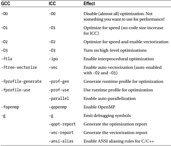
Revisit the compiler flags you used before the switch; you may have to remove some of them. Make sure that Intel Composer XE is invoked with the flags that give the best performance for your application (see Table 1-1). More information can be found in the Intel Composer XE documentation.6

Table 1-1. Selected Intel Composer XE Optimization Flags

GCC

ICC

Effect

-O0 -O0 Disable (almost all) optimization. Not

something you want to use for performance!

-O1 -O1 Optimize for speed (no code size increase

for ICC)

-O2 -O2 Optimize for speed and enable vectorization

-O3 -O3 Turn on high-level optimizations

-ftlo -ipo Enable interprocedural optimization

-ftree-vectorize -vec Enable auto-vectorization (auto-enabled with -O2 and -O3)

-fprofile-generate -prof-gen Generate runtime profile for optimization

-fprofile-use -prof-use Use runtime profile for optimization

-parallel Enable auto-parallelization

-fopenmp -qopenmp Enable OpenMP

-g -g Emit debugging symbols

-qopt-report Generate the optimization report

-vec-report Generate the vectorization report

-ansi-alias Enable ANSI aliasing rules for C/C++

(13)

For most applications, the default optimization level of -O2 will suffice. It runs fast and gives reasonable performance. If you feel adventurous, try -O3. It is more aggressive but it also increases the compilation time.

Tuning Intel MPI Library

If you have more time, you can try to tune Intel MPI parameters without changing the application source code.

Gather Built-in Statistics

Intel MPI comes with a built-in statistics-gathering mechanism. It creates a negligible runtime overhead and reports key performance metrics (for example, MPI to

computation ratio, message sizes, counts, and collective operations used) in the popular IPM format.7

To switch the IPM statistics gathering mode on and do the measurements, enter the following commands:

$ export I_MPI_STATS=ipm $ mpirun -np 16 xhpl

By default, this will generate a file called stats.ipm. Listing 1-1 shows an example of the MPI statistics gathered for the well-known High Performance Linpack (HPL) benchmark.8_{(We will return to this benchmark throughout this book, by the way.)}

GCC

ICC

Effect

-msse4.1 -xSSE4.1 Generate code for Intel processors with SSE 4.1 instructions

-mavx -xAVX Generate code for Intel processors with

AVX instructions

-mavx2 -xCORE-AVX2 Generate code for Intel processors with AVX2 instructions

-mcpu=native -xHost Generate code for the current machine used for compilation

(14)

Listing 1-1. MPI Statistics for the HPL Benchmark with the Most Interesting Fields Highlighted

Intel(R) MPI Library Version 5.0

Summary MPI Statistics Stats format: region Stats scope : full

############################################################################ #

# command : /home/book/hpl/./xhpl_hybrid_intel64_dynamic (completed) # host : esg066/x86_64_Linux mpi_tasks : 16 on 8 nodes # start : 02/14/14/12:43:33 wallclock : 2502.401419 sec # stop : 02/14/14/13:25:16 %comm : 8.43

# gbytes : 0.00000e+00 total gflop/sec : NA

#

############################################################################ # region : * [ntasks] = 16

#

# [total] <avg> min max # entries 16 1 1 1 # wallclock 40034.7 2502.17 2502.13 2502.4 # user 446800 27925 27768.4 28192.7 # system 1971.27 123.205 102.103 145.241 # mpi 3375.05 210.941 132.327 282.462

# %comm 8.43032 5.28855 11.2888

# gflop/sec NA NA NA NA # gbytes 0 0 0 0 #

#

# [time] [calls] <%mpi> <%wall>

# MPI_Send 2737.24 1.93777e+06 81.10 6.84 # MPI_Recv 394.827 16919 11.70 0.99 # MPI_Wait 236.568 1.92085e+06 7.01 0.59

(15)

From Listing 1-1 you can deduce that MPI communication occupies between 5.3 and 11.3 percent of the total runtime, and that the MPI_Send, MPI_Recv, and MPI_Wait

operations take about 81, 12, and 7 percent, respectively, of the total MPI time. With this data at hand, you can see that there are potential load imbalances between the job processes, and that you should focus on making the MPI_Send operation as fast as it can go to achieve a noticeable performance hike.

Note that if you use the full IPM package instead of the built-in statistics, you will also get data on the total communication volume and floating point performance that are not measured by the Intel MPI Library.

Optimize Process Placement

The Intel MPI Library puts adjacent MPI ranks on one cluster node as long as there are cores to occupy. Use the Intel MPI command line argument -ppn to control the process placement across the cluster nodes. For example, this command will start two processes per node:

$ mpirun -np 16 -ppn 2 xhpl

Intel MPI supports process pinning to restrict the MPI ranks to parts of the system so as to optimize process layout (for example, to avoid NUMA effects or to reduce latency to the InfiniBand adapter). Many relevant settings are described in the Intel MPI Library Reference Manual.9

Briefly, if you want to run a pure MPI program only on the physical processor cores, enter the following commands:

$ export I_MPI_PIN_PROCESSOR_LIST=allcores $ mpirun -np 2 your_MPI_app

If you want to run a hybrid MPI/OpenMP program, don’t change the default Intel MPI settings, and see the next section for the OpenMP ones.

If you want to analyze Intel MPI process layout and pinning, set the following environment variable:

$ export I_MPI_DEBUG=4

Optimize Thread Placement

If the application uses OpenMP for multithreading, you may want to control thread placement in addition to the process placement. Two possible strategies are:

$ export KMP_AFFINITY=granularity=thread,compact $ export KMP_AFFINITY=granularity=thread,scatter

The first setting keeps threads close together to improve inter-thread

(16)

Programs that use the OpenMP API version 4.0 can use the equivalent OpenMP affinity settings instead of the KMP_AFFINITY environment variable:

$ export OMP_PROC_BIND=close $ export OMP_PROC_BIND=spread

If you use I_MPI_PIN_DOMAIN, MPI will confine the OpenMP threads of an MPI process on a single socket. Then you can use the following setting to avoid thread movement between the logical cores of the socket:

$ export KMP_AFFINITY=granularity=thread

Tuning Intel Composer XE

If you have access to the source code of the application, you can perform optimizations by selecting appropriate compiler switches and recompiling the source code.

Analyze Optimization and Vectorization Reports

Add compiler flags -qopt-report and/or -vec-report to see what the compiler did to your source code. This will report all the transformations applied to your code. It will also highlight those code patterns that prevented successful optimization. Address them if you have time left.

Here is a small example. Because the optimization report may be very long, Listing 1-2 only shows an excerpt from it. The example code contains several loop nests of seven loops. The compiler found an OpenMP directive to parallelize the loop nest. It also recognized that the overall loop nest was not optimal, and it automatically permuted some loops to improve the situation for vectorization. Then it vectorized all inner-most loops while leaving the outer-most loops as they are.

Listing 1-2. Example Optimization Report with the Most Interesting Fields Highlighted

$ ifort -O3 -qopenmp -qopt-report -qopt-report-file=stdout -c example.F90

Report from: Interprocedural optimizations [ipo]

[...]

OpenMP Construct at example.F90(8,7)

remark #15059: OpenMP DEFINED LOOP WAS PARALLELIZED OpenMP Construct at example.F90(25,7)

remark #15059: OpenMP DEFINED LOOP WAS PARALLELIZED

(17)

LOOP BEGIN at example.F90(9,2)

remark #15018: loop was not vectorized: not inner loop

LOOP BEGIN at example.F90(12,5)

remark #25448: Loopnest Interchanged : ( 1 2 3 4 ) --> ( 1 4 2 3 )

remark #15018: loop was not vectorized: not inner loop

[...]

remark #25446: blocked by 125 (pre-vector)

remark #25444: unrolled and jammed by 4 (pre-vector) remark #15018: loop was not vectorized: not inner loop

remark #25446: blocked by 125 (pre-vector)

remark #25446: blocked by 128 (pre-vector)

remark #15003: PERMUTED LOOP WAS VECTORIZED

LOOP END

LOOP BEGIN at example.F90(14,7) Remainder

remark #25460: Loop was not optimized LOOP END

LOOP END LOOP END

[...]

LOOP END LOOP END LOOP END LOOP END LOOP END

(18)

remark #25446: blocked by 125 (pre-vector)

remark #25444: unrolled and jammed by 4 (pre-vector)

remark #15018: loop was not vectorized: not inner loop

[...]

LOOP END LOOP END LOOP END LOOP END LOOP END LOOP END

Listing 1-3 shows the vectorization report for the example in Listing 1-2. As you can see, the vectorization report contains the same information about vectorization as the optimization report.

Listing 1-3. Example Vectorization Report with the Most Interesting Fields Highlighted

$ ifort -O3 -qopenmp -vec-report=2 -qopt-report-file=stdout -c example.F90

[...]

(19)

LOOP END

[...]

LOOP END LOOP END

LOOP BEGIN at example.F90(15,8) Remainder

[...]

LOOP END

[...]

LOOP END

LOOP END LOOP END

[...]

LOOP END

LOOP END LOOP END LOOP END LOOP END

(20)

Use Interprocedural Optimization

Add the compiler flag -ipo to switch on interprocedural optimization. This will give the compiler a holistic view of the program and open more optimization opportunities for the program as a whole. Note that this will also increase the overall compilation time.

Runtime profiling can also increase the chances for the compiler to generate better code. Profile-guided optimization requires a three-stage process. First, compile the application with the compiler flag -prof-gen to instrument the application with profiling code. Second, run the instrumented application with a typical dataset to produce a meaningful profile. Third, feed the compiler with the profile (-prof-use) and let it optimize the code.

Summary

Switching to Intel MPI and Intel Composer XE can help improve performance because the two strive to optimally support Intel platforms and deliver good out-of-the-box (OOB) performance. Tuning measures can further improve the situation. The next chapters will reiterate the quick and dirty examples of this chapter and show you how to push the limits.

References

1. Intel Corporation, “Intel(R) MPI Library,” http://software.intel.com/en-us/ intel-mpi-library.

2. Intel Corporation, “Intel(R) Composer XE Suites,” http://software.intel.com/en-us/intel-composer-xe.

3. Argonne National Laboratory, “MPICH: High-Performance Portable MPI,” www.mpich. org.

4. Ohio State University, “MVAPICH: MPI over InfiniBand, 10GigE/iWARP and RoCE,” http://mvapich.cse.ohio-state.edu/overview/mvapich2/.

5. International Business Machines Corporation, “IBM Parallel Environment,” www-03.ibm.com/systems/software/parallel/.

6. Intel Corporation, “Intel Fortran Composer XE 2013 - Documentation,” http://software.intel.com/articles/intel-fortran-composer-xe-documentation/.

7. The IPM Developers, “Integrated Performance Monitoring - IPM,” http://ipm-hpc. sourceforge.net/.

8. A. Petitet, R. C. Whaley, J. Dongarra, and A. Cleary, “HPL : A Portable

Implementation of the High-Performance Linpack Benchmark for Distributed-Memory Computers,” 10 September 2008, www.netlib.org/benchmark/hpl/.

(21)

Overview of Platform

Architectures

In order to optimize software you need to understand hardware. In this chapter we give you a brief overview of the typical system architectures found in the high-performance computing (HPC) today. We also introduce terminology that will be used throughout the book.

Performance Metrics and Targets

The definition of optimization found in Merriam-Webster’s Collegiate Dictionary reads as follows: “an act, process, or methodology of making something (as a design, system, or decision) as fully perfect, functional, or effective as possible.”1_{To become practically}

applicable, this definition requires establishment of clear success criteria. These objective criteria need to be based on quantifiable metrics and on well-defined standards of measurement. We deal with the metrics in this chapter.

Latency, Throughput, Energy, and Power

Let us start with the most common class of metrics: those that are based on the total time required to complete an action–for example, the time it takes for a car to drive from the start to the finish on a race track, as shown in Figure 2-1. Execution (or wall-clock) time is one of the most common ways to measure application performance: to measure its

(22)

The runtime, or the period of time from the start to the completion of an application, is important because it tells you how long you need to wait for the results. In networking,

latency is the amount of time it takes a data packet to travel from the source to the destination; it also can be referred to as the response time. For measurements inside the processor, we often use the term instruction latency as the time it takes for a machine instruction entering the execution unit until results of that instruction are available—that is, written to the register file and ready to be used by subsequent instructions. In more general terms, latency can be defined as the observed time interval between the start of a process and its completion.

We can generalize this class of metrics to represent more of a general class of

consumable resources. Time is one kind of a consumable resource, such as the time allocated for your job on a supercomputer. Another important example of a consumable resource is the amount of electrical energy required to complete your job, called energy to solution. The official unit in which energy is measured is the joule, while in everyday life we more often use watt-hours. One watt-hour is equal to 3600 joules.

The amount of energy consumption defines your electricity bill and is a very visible item among operating expenses of major, high-performance computing facilities. It drives demand for optimization of the energy to solution, in addition to the traditional efforts to reduce the runtime, improve parallel efficiency, and so on. Energy optimization work has different scales; going from giga-joules (GJ, or 109_{joules) consumed at the application} level, to pico-joules (pJ, or 10–12_{joules) per instruction.}

One of the specific properties of the latency metrics is that they are additive, so that they can be viewed as a cumulative sum of several latencies of subtasks. This means that if the application has three subtasks following one after another, and these subtasks take times T₁, T₂ and T₃, respectively, then the total application runtime is T_app = T₁ + T₂ + T₃.

Other types of metrics describe the amount of work that can be completed by the system per unit of time, or per unit of another consumable resource. One example of car performance would be its speed defined as the distance covered per unit of time; or of its fuel efficiency, defined as the distance covered per unit of fuel—, such as miles per gallon. We call these metrics throughput metrics. For example, the number of instructions per second (IPS) executed by the processor, or the number of floating point operations per second (FLOPS) are both throughput metrics. Other widely used metrics of this class are memory bandwidth (reaching tens and hundreds of gigabytes per second these days), and network interconnection throughput (in either bits per second or bytes per second). The unit of power (watt) is also a throughput metric that is defined as energy flow per unit of time, and is equal exactly to 1 joule per second.

(23)

You may encounter situations where throughput is described as the inverse of latency. This is correct only when both metrics describe the same process applied to the same amount of work. In particular, for an application or kernel that takes one second to complete 109_{arithmetic operations on floating point numbers, it is correct to state that its} throughput is 1 GFLOPS (gigaFLOPS, or 109_FLOPS).

However, very often, especially in computer networks, latency is understood as the time from the beginning of the packet shipment until the first data arrives at the destination. In this context, latency will not be equal to the inverse value of the throughput. To grasp why this happens, compare sending a very large amount of data (say, 1 terabyte (TB), which is 1012_{bytes) using two different methods}2_:

1. Shipping with overnight express mail 2. Uploading via broadband Internet access

The overnight (24-hour) shipment of the 1TB hard drive has good throughput but lousy latency. The throughput is (1 × 1012_{× 8) bits / (24 × 60 × 60) seconds = about 92} million bits per second (bps), which is comparable to modern broadband networks. The difference is that the overnight shipment bits are delayed for a day and then arrive all at once, but the bits we send over the Internet start appearing almost immediately. We would say that the network has much better latency, even though both methods have approximately the same throughput when considered over the interval of one day.

Although high throughput systems may have low latency, there is no causal link. Comparing a GDDR5 (Graphics Double Data Rate, version 5) vs. DDR3 (Double Data Rate, type 3) memory bandwidth and latency, one notices that systems with GDDR5 (such as Intel Xeon Phi coprocessors) deliver three to five times more bandwidth, while the latency to access data (measured in an idle environment) is five to six times lower than in systems with DDR3 memory.

Finally, a graph of latency versus load looks very different from a graph of throughput versus load. As we will see later in this chapter, memory access latency goes up

exponentially as the load increases. Throughput will go up almost linearly at first, then levels out to become nearly flat when the physical capacity of the transport medium is saturated. Simply by looking at a graph of test results and keeping those features in mind, you can guess whether it is a latency graph or a throughput graph.

(24)

Cantrill and Bonwick describe three fundamental ways of using concurrency to improve application performance.3_{At the same time, these three ways represent the}

typical optimization targets for either latency or throughout metrics: • Increase throughput: By executing multiple tasks concurrently,

the general system throughput can be increased.

• Reduce latency: A given amount of work is completed in shorter time by dividing it into parts that can be completed concurrently. • Hide latency: Multiple long-running tasks are executed in

parallel by the underlying system. This is particularly effective when some tasks are blocked (for example, if they must wait upon disk or network I/O operations), while others can proceed independently.

Peak Performance as the Ultimate Limit

Every time we talk about performance of an application running on a machine, we try to compare it to the maximum attainable performance on that specific machine, or peak performance of that machine. The ratio between the achieved (or measured) performance and the peak performance gives the efficiency metric. This metric is often used to drive the performance optimization, for an increase in efficiency will also lead to an increase in performance according to the underlying metric. For example, efficiency for the wall-clock time is the fraction of time that is spent doing useful work, while efficiency for throughout is a measure of useful capacity utilization.

Consider the example of how to quantify efficiency for a network protocol. Network protocols normally require each packet to contain a header and a footer. The actual data transmitted in the packet is then the size of the packet minus the protocol overhead. Therefore, efficiency of using the network, from the application point of view, is reduced from the total utilization according to the size of the header and the footer. For Ethernet, the frame payload size equals 1536 bytes. The TCP/IP header and footer take 40 bytes extra. Hence, efficiency here is equal to 1536 / 1576 × 100, or 97.5 percent.

Understanding the limitations of maximum achievable performance is an important step in guiding the optimization process: the limits are always there! These limits are driven by physical properties of the available materials, maturity of the technology, or (trivially) the cost. Particularly, the propagation of signals along the wires is limited by the speed of light in the respective material. Thus, the latency for completing any work using electronic equipment will always be greater than zero. In the same way, it is not possible to build an infinitely wide highway, for its throughput will always be limited by the number of lanes and their individual throughputs.

(25)

Scalability and Maximum Parallel Speedup

The ability to increase performance by using more resources in parallel (for example, more processors) is called scalability. The basic approach in high-performance

computing is to use many computational resources in parallel to solve one problem, and to add still more resources if higher performance is required. Scalability analysis indicates how efficient an application is using the increasing numbers of parallel computing elements, such as cores, vector units, memory, or network connections.

Increase in performance before and after addition of the resources is called speedup. When talking about throughput-related metrics, speedup is expressed as the ratio of the throughput after addition of the resources versus the original throughput. For latency metrics, speedup is the ratio between the original latency and the latency after addition of the resources. This way speedup is always greater than 1.0 if performance improves. If the ratio goes below 1.0, we call this negative speedup, or simply slowdown.

Amdahl’s Law, also known as Amdahl’s argument,4_{is used to find the maximum}

expected improvement for an entire application when only a part of the application is improved. This law is often used in parallel computing to predict the theoretical maximum speedup that can be achieved by adding multiple processors. In essence, Amdahl’s Law says that speedup of a program using p processors in parallel is limited by the time needed for the nonparallel fraction of the program (f ), according to the following formula:

Speedup p

f p

£

+ ×

-1 ( 1)

where f takes values between 0 and 1.

(26)

It may be depressing to realize that the maximum possible speedup will be limited by something you can’t improve by adding more resources. Even so, consider the same speedup problem from another angle: what happens if the amount of work in the parallelizable part of the execution can be increased?

If the relative share of time taken by the serial portion of the application remains unchanged with the increase of the workload size, there is no inherent speedup factor available, and as illustrated in Figure 2-4 (left), Amdahl’s Law still works. However, John Gustafson observed that there was significant speedup opportunity available if the serial component shrank in size relative to the parallel part as the amount of data processed by the application (and consequently the amount of computation) expanded.5

Figure 2-4. Illustration of Gustafson’s observation

(27)

This observation leads to two kinds of scalability metrics:

• Strong scaling: How performance varies with the number of computing elements for a fixed total problem size. In strong scaling, perfect scaling (i.e., when performance improves linearly) is achieved when speedup is equal to the number of computing elements involved.

• Weak scaling: How performance varies with the number of computing elements for a fixed problem size per processor, and additional computing elements are used to solve a larger total problem. In the case of weak scaling, perfect scaling is achieved if the runtime remains constant while the workload is increased proportionally to the number of computing elements involved.

Bottlenecks and a Bit of Queuing Theory

Performance analysis is a process of identifying bottlenecks and removing them, with the objective of increasing overall application performance. Certain parts of the application that limit performance of the entire application are called performance bottlenecks. The significance of the term bottleneck can be illustrated with the same car metaphor that we have used before (see Figure 2-5). When there is a toll gate on the road that can process only one car at a time, the rate at which cars will pass along the highway (that is, highway throughput) is limited by the width of the toll gate, irrespective of how many more lanes are on the road before and after it. In other words, the toll gate is a bottleneck. By increasing the width of the toll gate, it is possible to increase the rate of cars on the highway.

Figure 2-5. Bottlenecks on the road are commonly known as traffic jams

As shown in Figure 2-5, bottlenecks can create traffic jams on the highway. Using the terminology of queuing theory,6_{we are talking about the toll gate as a single service}

(28)

This approach is widely used by queuing network modeling, where a computer system is represented as a network of queues—that is, a collection of service centers that represent system resources and customers who represent users or transactions. This model provides a framework for gathering, organizing, evaluating, and understanding information about the computer system, as well as for identifying possible bottlenecks and testing ideas for system improvement. Such models are widely used for quantitative analysis during computer system design and the application development process.

Roofline Model

Amdahl’s law and the queuing network models both offer “bound and bottleneck analysis,” and they work quite well in many cases. However, both complexity and the level of concurrency of modern high-performance systems keep increasing. Indeed, even smartphones today have complex multicore chips with pipelines, caches, superscalar instruction issue, and out-of-order execution, while the applications increasingly use tasks and threads with asynchronous communication between them. Quantitative queuing network models that simulate behavior of very complex applications on modern multicore and heterogeneous systems have become very complex. At the same time, the speed of microprocessor development has outpaced the speed of the memory evolution; and in most cases, specifically in high-performance computing, the bandwidth of the memory subsystem is often the main bottleneck.

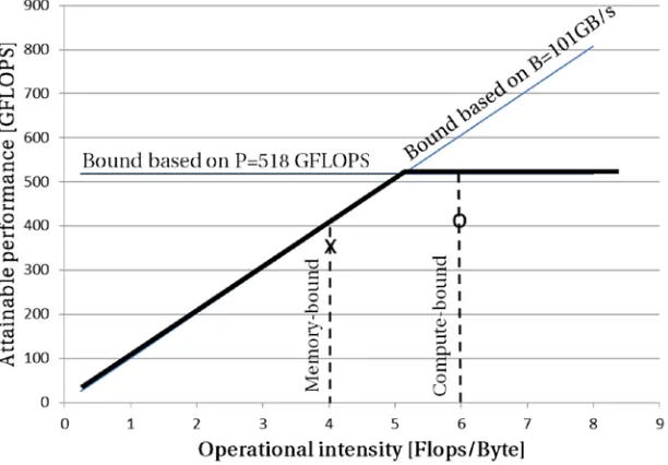
In search of a simplified model that would relate processor performance to the off-chip memory traffic, Williams, Waterman, and Patterson observed that that “the Roofline [model] sets an upper bound on performance of a kernel depending on the kernel’s operational intensity.”7_The_{Roofline model}_{subsumes two platform specific}

ceilings in one single graph: floating-point performance and memory bandwidth. The model, despite its apparent simplicity, provides an insightful visualization of the system bottlenecks. Peak floating point and memory throughput performances can usually be found from the architecture specifications. Alternatively, it is possible to find sustained memory performance by running the STREAM benchmark.8

(29)

The horizontal line shows peak performance of the computer. This is a hardware limit for this server. The X-axis represents amount of work (in number of floating point operations, or Flops) done for every byte of data coming from memory: Flops/byte (here, “Flops” stands for the plural of “Flop”–the number of floating point operations, rather than FLOPS, which is Flops per second). And the Y-axis represents gigaFLOPS (109 FLOPS), which is a throughput metric showing the number of floating point operations executed every second (Flops/second, or FLOPS). With that, taking into account that

bytes second Flops second Flops byte

/ /

/

= , the memory throughput metric gigabytes/second is

represented by a line of unit slope in Figure 2-6. Thus, the slanted line shows the maximum floating point performance that the memory subsystem can support for the given operational intensity. The following formula drives the two performance limits in the graph shown in Figure 2-6:

Attainable performance GLOPS

Peak floating po performan

[ ]

min

= int cce

Peakmemory bandwidth Operational ensity

, ´

ì í î

ü ý þ

int

(30)

compute-bound. For another kernel (the one marked by “X”), any improvement will eventually hit the slanted part of the roof, meaning its performance is ultimately memory bound. The roofline found for a specific system can be reused repeatedly for classifying different kernels.

Performance Features of Computer Architectures

We have discussed the major types of performance characteristics and approaches to estimate maximum attainable performance. Let’s turn to a discussion of where the potential performance increases can come from.

Increasing Single-Threaded Performance: Where You

Can and Cannot Help

We will refer to the basic execution context as a thread—a sequence of machine instructions executed by a processor core. Typically, a thread is the smallest context of execution that is independently managed by the operating system (OS). A thread can be granted a processor core to execute instructions on, or it can be put to sleep to free execution resources for other threads in a queue. Under Linux OS, the most widely used operating system in HPC these days,9_{kernel threads and processes are the same entity: simply a runable task. Later, when}

we talk about hybrid programing, we will want to distinguish processes and threads. But for now let us leave them as a software thread or task, understanding that at any given moment each processor core executes instructions from a single task. Making these instructions run faster is the essence of application optimization.

Performance of a single thread can be defined by number of instructions executed per second (IPS) and calculated as a product of two values (IPS = CPS × IPC):

1. Number of processor clock cycles per second (CPS). It is more often called processor clock frequency, or simply frequency, and is measured in Hertz (Hz), or for most processors in gigaHertz (GHz), which is 109_Hertz.

2. Number of instructions executed per processor clock tick,

instructions per cycle (IPC).

An application usually cannot do anything about the processor frequency: it is something defined at the manufacturing time and considered fixed or at least not directly changeable when an application is running. In contrast, the IPC is a function of both the processor microarchitecture and your application. The microarchitecture is an internal implementation of the processor. Very simple microarchitectures can execute a maximum of only one instruction per cycle; they are called scalar. More sophisticated ones can execute concurrently several instructions at every clock cycle and are known as superscalar.

(31)

demanding customers. Superscalar microarchitectures that are predominant among high-performance focused processors these days provide a much needed solution to the frequency problem. Modern x86 superscalar processors (such as the Intel Core family) can complete up to four instructions per cycle, so it would be as if the frequency was effectively increased four times in a scalar processor. This book was written using a computer with 2.5 GHz Intel Core i5 processor. If it were written on a scalar processor, such as the older Intel 486, the processor would need to run at approximately 10 GHz to be equal in peak performance.

Superscalar execution provides a great way to improve application performance. However, it is to a large extent simply a capability of the processor that needs to be exploited to yield real benefit in application performance. When we talk about microarchitecture optimization in Chapter 7, we review cases when a superscalar processor does not execute as many instructions as it could, and how to fix that. But before we go any further, it is important to note that very often during the optimization process we use a multiplicative inverse of IPC called CPI, or clocks per instruction . With some simplification we can use the relationship CPI = 1 / IPC without losing many details. Many performance profiling tools (such as Intel VTune Amplifier XE,10_{discussed in}

greater details in Chapters 6 and 7) use CPI instead of IPC to make it easier to correlate observed CPI metrics with table data on latencies that are traditionally provided for each instruction in processor cycles.

It is important to familiarize yourself with both metrics and be able to assess their values. For example, when a profiler tells you that the average CPI is equal to 2 (meaning it takes two cycles on average to complete every instruction), that means IPC is equal to 0.5 (or one instruction completed every two processor cycles). This level of performance would be rather bad for a modern processor that can (theoretically) reach 4 IPC (delivering results for four instructions every cycle) and the best achievable average CPI of 0.25. Luckily, such an application or piece of code under consideration provides great opportunity for optimization.

Process More Data with SIMD Parallelism

Another way to increase performance of each thread is to look at the data being processed. So far we have only discussed the limit of each processor core with respect to the instructions, but not with respect to the data each instruction works with. The next natural way to optimize an application execution is to let each instruction deal with more than one element of data at a time. Michael J. Flynn gave this approach the name SIMD, standing for Single Instruction Multiple Data single instruction, multiple data.11_{As it}

(32)

Following this principle, the SIMD vector instruction sets implement not only basic arithmetic operations (such as additions, multiplications, absolute values, shifts, and divisions) but also many other useful instructions present in nonvectorized instruction sets. They also implement special operations to deal with the contents of the vector registers—for example, any-to-any permutations—and gather instructions that are useful for vectorized code that accesses nonadjacent data elements.

SIMD extensions for the x86 instruction set were first brought into the Intel architecture under the Intel MMX brand in 1996 and were used in Pentium processors. MMX had a SIMD width of 64 bits and focused on integer arithmetic. Thus, two 32-bit integers, or four 16-bit integers (as type short in C), or eight 8-bit integer numbers (C type char), could be processed simultaneously. Note also that the MMX instruction set extensions for x86 supported both signed and unsigned integers.

New SIMD instruction sets for x86 processors added support for new operations on the vectors, increased the SIMD data width, and added vector instructions to process floating point numbers much demanded in HPC. In 1999, SIMD data width was increased to 128 bits with SSE (Streaming SIMD Extensions), and each SSE register (called xmm) was able to hold two double precision floating point numbers or two 64-bit integers, four single precision floats or four 32-bit integers, eight 16-bit integers or 16 single-byte elements.

In 2008, Intel announced doubling of the vector width to 256 bits in Intel AVX (Advanced Vector eXtensions) instruction set. The extended register was called ymm. The

(33)

The latest addition to Intel AVX, announced in 2013, includes definition of Intel Advanced Vector Extensions 512 (or AVX-512) instructions. These instructions represent a leap ahead to the 512-bit SIMD support (And guess what? The registers are now called zmm). Consequently, up to eight double precision or 16 single precision floating point numbers, or eight 64-bit integers, or 16 32-bit integers can be packed within the 512-bit vectors. Figure 2-9 shows the relative sizes of SSE, AVX, and AXV-512 SIMD registers with highlighted packed 64-bit data types (for instance, double precision floats).

Figure 2-8. AVX registers and supported packed data types

(34)

Now that you’re familiar with the important concepts of SIMD processing and superscalar microarchitectures, the time has come to discuss in greater detail the FLOPS (floating point operations per second) metric, one of the most cited HPC performance metrics. This measure of performance is widely used as a performance metric in the field of scientific computing where heavy use of calculations with the floating point numbers is very common. The last “S” designates not the plural form for FLOP but a ratio “per second” and is historically written without a slash (/) and avoiding double “S” (i.e., FLOPS instead of Flops/S). In our book we will stick to the common practice. In some situations, we will need to refer to floating point operations, so abbreviate it as Flops and produce required ratios as needed. For example, we will write Flops/cycle when there is a need to count number of floating point operations per processor cycle of the processor core.

One of the most often quoted metrics for individual processors or complete HPC systems is their peak performance. This is the theoretically maximum possible performance that could be delivered by the system. It is defined as follows:

Peak performance of a system is a sum of peak performances of •

all computing elements (namely, cores) in the system.

Peak performance for a vectorized superscalar core is calculated •

as the number of independent floating point arithmetic operations that the core can execute in parallel, multiplied by the number of vector elements that are processed in parallel by these operations.

As an example, if you have a cluster of 16 nodes, each with a single Intel Xeon E3-1285 v3 processor that has four cores with Haswell microarchitecture running at 3.6 GHz, it will have peak performance of 3686.4 gigaFLOPS (or 109_{FLOPS). Using the FMA} (fused multiply add, which is b = a × b + c ) instruction, a Haswell core can generate four Flops/cycle (via execution of two FMAs per cycle) with a SIMD vector putting out four results per cycle, thus delivering peak performance of 57.6 gigaFLOPS at

the frequency of 3.6 GHz: 4Flops 4 3 6 57 6

cycle´ SIMD´ . GHz= . GFLOPS. Multiplying this by

total number of cores in the cluster (64 16= nodes´1processor´4 )

node

cores

processor gives

3686.4 gigaFLOPS, or 3.68 teraFLOPS.

(35)

Distributed and Shared Memory Systems

So far we have discussed how application performance can be improved by increasing the amount of work done in parallel inside a processor core: by allowing more

instructions to execute in parallel in superscalar microarchitectures, and by making each instruction process more data using the SIMD paradigm. As the next step we discuss two types of parallelism that can be employed to further enhance application performance. The main difference visible to you as a software developer is how the memory is shared and accessed by the processors. In the shared memory approach, multiple application threads can access all the memory simultaneously in a transparent. In the distributed memory approach, there is local and remote memory, and in order to work on any piece of data, that data has to be first copied into the local memory of the thread or process.

Use More Independent Threads on the Same Node

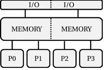
The first approach we will discuss harnesses several threads belonging to one program that can simultaneously access the same memory locations. Application threads can communicate through this shared memory with each other and avoid redundant copies of data. Shared memory is an efficient means of passing data between program threads. To connect multiple processors (each with multiple cores), the underlying system needs to have robust hardware to support arbitration and ordering of the memory requests.

In a shared memory system, the memory is presented to the application as a uniform, contiguous address range, while in fact the cost of accessing different parts of the memory by different processors may not be the same. Since most modern high-performance processors contain integrated memory controllers, there is some memory attached to each processor that is called local memory of that processor. Memory attached to other processors in the same system then needs to be accessed through an internal interconnect, such as Intel QuickPath Interconnect (QPI), that provides hardware mechanisms for all memory in the system to appear as one contiguous address space. There may be additional latency associated with accessing this remote memory

over the latency for accessing the local memory. Shared memory systems that have this extra latency are called Non-Uniform Memory Access (NUMA) systems.

Impact from NUMA can be characterized by the ratio between the latencies for remote and local memory access. This ratio is called the NUMA factor. For example, in a dual-processor server with Intel Xeon E5-2697 v2 processors, local memory access latency (measured in the idle case) is around 50-70 ns (nanoseconds, or 10-9_second), while for remote memory access latency is equal to 90-110 ns, which leads to the NUMA factor for this system of approximately 1.5. The larger the shared memory system is, the larger the NUMA factor normally becomes. In fact, you may even find several different NUMA factors within larger systems. As a result, it is more difficult to optimize applications for these systems.

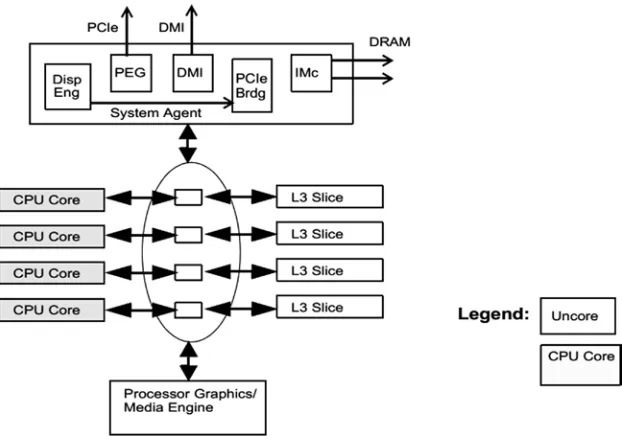
A generic diagram of a shared memory system in Figure 2-10 shows four processors,

(36)

To get details on the NUMA topology of your system, use the numactl tool that is available for all major Linux distributions. On our workstation, the execution of numactl

tool with the --hardware argument displays the following information (see Listing 2-1):

Listing 2-1. Output of the numactl --hardware Command

available: 2 nodes (0-1)

node 0 cpus: 0 1 2 3 4 5 6 7 8 9 10 11 24 25 26 27 28 29 30 31 32 33 34 35 node 0 size: 65457 MB

node 0 free: 57337 MB

node 1 cpus: 12 13 14 15 16 17 18 19 20 21 22 23 36 37 38 39 40 41 42 43 44 45 46 47

node 1 size: 65536 MB node 1 free: 59594 MB node distances: node 0 1 0: 10 21 1: 21 10

The output of the numactl tool shows two NUMA nodes, each with 24 processors (and just a hint-these are twelve physically independent cores with two threads each), and 64 GB of RAM per NUMA node, or 128 GB in the server in total.

In a similar manner to physical memory, the Input/Output subsystem and the I/O controllers are shared inside the multiprocessor systems, so that any processor can access any I/O device. Similarly to memory controllers, the I/O controllers are often integrated into the processors, and latency to access local and remote devices may differ. However, since latency associated with getting data from or to external I/O devices is significantly higher than the latency added by crossing the inter-processor network (such as QPI), this additional inter-processor network latency can be ignored in most cases. We will discuss specific I/O related issues in greater detail in Chapter 4.

Don’t Limit Yourself to a Single Server

Unfortunately, there are practical limits to the size of a single system with shared memory, mostly driven by cost of building the hardware, as well as by overheads associated with the memory arbitration logic.

(37)

To achieve higher performance than a single shared memory system could offer, it is more beneficial to put together several smaller shared memory systems, and interconnect those with a fast network. Such interconnection does not make the memory from different boxes look like a single address space. This leads to the need for software to take care of copying data from one server to another implicitly or explicitly. Figure 2-11 shows an example system.

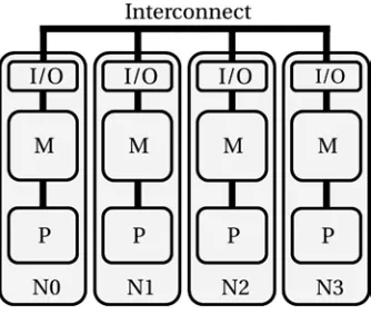
Figure 2-11. Diagram of a distributed memory system

Figure 2-11 shows a computer with four nodes, N0–N3, interconnected by a network, also called interconnect or fabric. Processors in each node have their own dedicated private memory and their own private I/O. In fact, these nodes are likely to be shared memory systems like those we have reviewed earlier. Before any processor can access data residing in another node’s private memory, that data should be copied to the private memory of the node that is requesting the data. This hardware approach to building a parallel machine is called distributed memory. The additional data copy step, of course, has additional penalty associated with it, and the performance impact greatly depends on characteristics of the interconnect between the nodes and on the way it is programmed.

HPC Hardware Architecture Overview

(38)

A Multicore Workstation or a Server Compute Node

Let us start with an overview of a simple workstation or a desktop computer. It has at least one processor and that processor very likely has multiple cores.

A core is an independent piece of hardware that does not share any hardware resources with other cores inside the processor. The core executes instructions of a computer program by performing requested arithmetical, logical, input/output, and other operations. Supported instructions are usually hardwired into the cores. They are called the instruction set. This is the language that the processor speaks, and it won’t understand a different one. All instructions for mainstream Intel processors are based on the x86 instruction set, with multiple extensions, known as MMX, SSE, AES-NI, AVX, etc. The supported instruction set and the architecture state (including all the registers visible to the instructions, flags, etc.) define a core architecture.

Optimizing HPC Applications with Intel Cluster Tools