A SIMPLE AND FAST CONTOUR
PLOTTING ALGORITHM
FOR LINEAR 2D AND 3D ELEMENTS
CHANDAN SINGH
Department of Computer Science, Punjabi University, Patiala, 147 002, India.
JASWINDER SINGH SAINI
Department of Mechanical Engineering, Thapar University, Patiala, 147004, India.
Abstract:
We present a fast contour plotting algorithm using three-node triangular and four-node tetrahedral elements which are mostly used in FEA as they fit better in an irregular domain. To make the overall task simple the analysis is performed with higher order elements whereas the graphical display of results in the form of contour lines or surfaces is carried out with linear elements. A three-node triangular and four-node tetrahedral element which interpolates the function linearly over the element is used mainly for its simplicity for fast contouring. A fast algorithm using the shape functions is demonstrated for the plotting of contours. Numerical results are presented using these elements.
Keywords: FEA; Contour Plotting; three-Node triangle; four-Node tetrahedral; Linear Interpolation.
1. Introduction
Graphical representation of results is essential to understand numerical model behavior. This representation substitutes analysis of a large amount of data by a simple visual inspection. Contour plotting of data is one step towards such representation. A contour plot is a curve along which the physical parameter has a constant value in a given domain.
coordinates which are mapped to global coordinates and finally converted into screen coordinates for display purpose. This is a direct approach and works well but it is computation intensive. Moreover, contour surfaces are not generated in explicit form but, only the contour points are located. A smooth contour surfaces is generated within the volume of an element using marching cubes method and bi-cubic polynomials [Gallagher and Nagtegaal (1989)]. Marching cubes algorithm is also used for tetrahedral, prism and hexahedral elements to create contour surfaces [Breitkopf (1998)]. The more complex forms and higher-order elements were treated by subdivision into these simple forms. Linear interpolation is used within the element providing exact tracing of contours for linear shape functions. A contour surfaces is generated using quadratic tetrahedrals by finding the intersection of a contour surface with each face of a tetrahedron and then connecting the face intersection curves end-to-end to form group of curves that bound various portions of the contour surface [Wiley et al. (2003)]. After determining the bounding curves, the contour surface is developed using Bernstein’s polynomials. The method generates very smooth contour surfaces but due to approximation involved the points on contour surface deviate from their true locations.
From the above discussion it is seen that contouring in 2D and 3D is targeted towards generating accurate and smooth contour surfaces. These two objectives are conflicting in nature. Often, for simplicity the higher order elements are decomposed to lower order elements at the cost of accuracy. A simplest way to plot contours on 2D and 3D domains is to use linear interpolation over triangular and tetrahedral elements. As stated earlier, a three-node triangular and four-node tetrahedral element which interpolates the function linearly over the element is used mainly for its simplicity for fast contouring. In the present work an attempt is made to develop a very fast algorithm for plotting linear contours over three-node triangular and four-node tetrahedral elements.
2. Mathematical Formulations
A contour in 2D is a continuous curve characterized by the equation
f
(
x
,
y
)
=
C
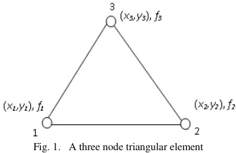
(1) where x,y are spatial coordinates and C is a constant.A three node triangular element normally used for analysis is given in Fig. 1.
Fig. 1. A three node triangular element
The coordinates of the three vertices of the triangle are available prior to analysis and the physical quantity,
f(x,y), is known after analysis, i.e. after solving a mathematical model. The linear interpolation of coordinates and functions over the element is performed as
∑
=
=
3
1
i i i
x
N
x
(2)
∑
=
=
3
1
i i i
y
N
y
(3)
∑
=
=
3
1
)
,
(
i i i
f
N
y
x
f
(4)where, ܰ= ܮ and
L
(
a
b
x
c
y
)
i i ii
+
+
∆
=
2
1
(5)
The coefficients ai ,biand ciare cofactors of the matrix, M, where
=
3 3
2 2
1 1
1
1
1
y
x
y
x
y
x
and,
∆
=
det
( )
M
. The functionsL
i=
L
i(
x
,
y
)
,
i
=
1
,
2
,
3
are called shape functions.The Eq. (4) is simplified to
C
y
l
x
l
l
0+
1+
2=
(7) where(
1 1 2 2 3 3)
0 2 1 f a f a f a
l + + ∆
=
(
1 1 2 2 3 3)
1 2 1 f b f b f b
l + + ∆
=
(
1 1 2 2 3 3)
2 2 1 f c f c f c
l + + ∆
=
Eq. (7) can be compared with the following general equation which represents a line
(
x
y
z
)
ax
by
c
F
,
,
=
+
+
(8) The problem now reduces to accurately trace the contour represented by a line over a triangle. The high speed line algorithm like mid-point algorithm [Hearn and Baker (2003)] is used to trace the line.Now, for a four-node tetrahedral element, the contour Eq. (1) in 3D assumes the following form
C
z
y
x
f
(
,
,
)
=
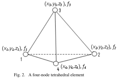
(9) where x, y, z are spatial coordinates and C is a constant.A four node tetrahedral element normally used for analysis is given in Fig. 2.
Fig. 2. A four-node tetrahedral element
The coordinates of the four vertices of the tetrahedral are available prior to analysis and the physical quantity,
f(x,y,z), is known after analysis, i.e. after solving a mathematical model. The linear interpolation of coordinates and functions over the element is performed as
∑
==
4 1 i i ix
N
x
(10)
∑
==
4 1 i i iy
N
y
(11)
∑
==
4 1 i i iz
N
z
(12)
∑
==
4 1)
,
,
(
i i if
N
z
y
x
f
(13)where, where, ܰ = ܮ and
L
(
a
b
x
c
y
d
z
)
i i i ii
+
+
+
∆
=
6
1
(14)
=
p p p m m m j j j i i iz
y
x
z
y
x
z
y
x
z
y
x
M
1
1
1
1
(15)and,
6
∆
=
det
( )
M
. The functionsL
i=
L
i(
x
,
y
,
z
)
,
i
=
1
,
2
,
3
,
4
are called shape functions. The Eq. (13) is simplified toC
z
l
y
l
x
l
l
0+
1+
2+
3=
(16)where
(
1 1 2 2 3 3 4 4)
0 6 1 f a f a f a f a
l + + + ∆
=
(
1 1 2 2 3 3 4 4)
1 6 1 f b f b f b f b
l + + + ∆
=
(
1 1 2 2 3 3 4 4)
2 6 1 f c f c f c f c
l + + + ∆
=
(
1 1 2 2 3 3 4 4)
3 6 1 f d f d f d f d
l + + + ∆
=
Eq. (16) can be compared with the following general equation which represents a plane
(
x
y
z
)
ax
by
cz
d
F
,
,
=
+
+
+
(17) The problem now reduces to accurately trace the contour represented by a plane over a tetrahedral.3. Contouring Algorithm
The overall algorithm for contouring is described as follows. (i) Consider an element.
(ii) Find the minimum and the maximum, fmin and fmax, of f(x, y, z) over the element. (iii) If
f
min≤
C
≤
f
maxthen go to step (iv), else go to step (vi).(iv) Trace the contour over the element. (v) Save the contour.
(vi) If not all the elements are processed, then consider the next element and go to step (ii), else go to step (vii).
(vii) Join the contours of the same level. (viii) Plot the contours.
Except for step iv) all steps are easy to understand. Detailed explanation is given for this step as follows.
3.1 Tracing contour line over a triangle element
The contour line is traced over the triangle element by finding the possible intersection of the line with the edge of the triangle.
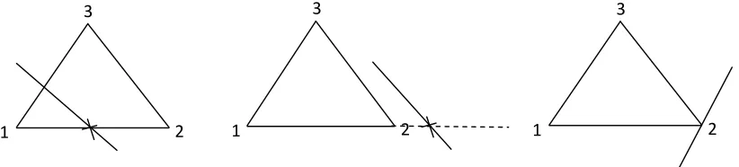
Fig. 3. Possible cases of intersection of a side with nodes 1 and 2 with the line a) The line intersects at one point of the side; b) Intersection point is outside the side; c) The line touches the corner point
The intersection of a line with one of the sides of the triangle has three possible cases as shown in Fig. 3(a) through Fig. 3(c). In the second case the contour line lies outside the element. The last case, if detected, is discarded for contour plotting as it yields a single point which is of no interest.
In general, we find intersection of a line with an edge of a triangle using parametric equations and record the point of intersection, if any. Let the parametric equation in vector form of an edge represented by
P
1P
2end points be
P
=
P
1+
u
(
P
2−
P
1)
(18) And the general equation of the contour line be
l
1x
+
l
2y
+
l
3=
0
(19) On substituting x and y from Eq. (18) into Eq. (19) and rearranging, we get
(
)
(
(
)
(
)
)
2 1 2 2 1 1 3 1 2 1 1
y
y
l
x
x
l
l
y
l
x
l
u
−
+
−
+
+
=
(20)The intersection point lies between
P
1 andP
2if the value of u lies between 0 to 1.Similarly, the intersection points on all the edges are calculated and joined with the help of a line to form a contour line over an element.
3.2 Tracing contour surface over a tetrahedral element
As is discussed in 2D, we find intersection of an edge of a tetrahedral with the contour plane using parametric equations and record the point of intersection, if any. Let the parametric equation in vector form of an edge represented by
P
1P
2end points be
P
=
P
1+
u
(
P
2−
P
1)
(21) And the general equation of the contour plane be
l
1x
+
l
2y
+
l
3z
+
l
4=
0
(22) On substituting x, y and z from Eq. (18) into Eq. (19) and rearranging, we get
(
)
(
(
)
(
)
(
)
)
2 1 3 2 1 2 2 1 1 4 3 1 2 1 1
z
z
l
y
y
l
x
x
l
l
z
l
y
l
x
l
u
=
+
+
+
−
+
−
+
−
(23)The intersection point lies between
P
1 andP
2if the value of u lies between 0 to 1.Similarly, the intersection points on all the edges are calculated and joined with the help of a line to form a contour plane over an element. The shading of the plane is done using OpenGL.
4. Implementation of the Algorithm and Experimental Results
The contour plot algorithm is implemented in Turbo C++ and runs on an IBM compatible PC under Windows operating system. The algorithm takes 0.054945 sec for the tracing and plotting of contours for 276, four-node tetrahedral elements on a PC with 3.0 GHz CPU and 256 RAM. The OpenGL graphics libraries are used to display the geometry and contour surfaces.
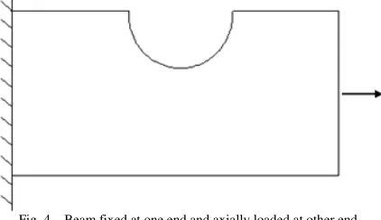
The first problem is a deflection of a 2D beam with length 400 mm, height 200 mm, and upper cut of 40 mm radius. The beam is fixed at one end and an axial load is applied at the other end, shown in Fig. 4.
Fig. 4. Beam fixed at one end and axially loaded at other end
For a load of 100 N, Young’s Modulus
2
.
1
×
10
5N/mm2, Poisson’s ratio 0.3, the values of deflections are derived using FEA taking 132, three-node triangle elements, considering the problem as 2D plane problem with negligible thickness of beam 0.5 mm.
E
A
WL
x
x
=
δ
where W is the load applied, L is the length of beam, Ax is the area of cross section and E is the Young’s Modulus.
The resultant horizontal deflections are considered for contouring in the numerical experimentation for the proposed algorithm. Fig. 5 depicts the contour plots of horizontal deflections using three-node triangles for different levels of deflections.
Fig. 5. Contour plot of horizontal deflection using three-node triangles for axially loaded beam (All units in mm )
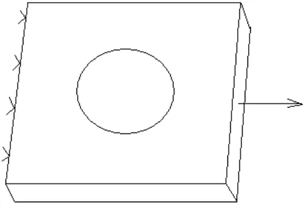
The second problem is a deflection of a 3D beam with length 10 mm, height 10 mm, thickness 1 mm and central through hole of 5 mm diameter. The beam is fixed at one end and an axial load is applied at the other end, shown in Fig. 6. For a load of 48 N, Young’s Modulus
200
GPa
, Poisson’s ratio 0.3, the values of horizontal deflections are derived using FEA taking 274, four-node tetrahedral elements.Fig. 6. Beam fixed at one end and axially loaded at other end
Fig. 7. Contour surfaces of horizontal deflection using four-node tetrahedrals for the different deflection levels (All units in mm)
5. Conclusions
A number of 2D and 3D problems in engineering applications are analyzed using triangular and tetrahedral elements respectively because they fit better in an irregular shape as compared to other elements. Algorithms for fast contour plotting using three-node triangular elements and four-node tetrahedral elements are discussed in this paper. The interpolation functions representing contours in 2D and 3D elements are degenerated into lines and planes respectively. It is observed that the contouring algorithm is very fast and takes 0.054945 sec for the problem involving 276, four-node tetrahedral elements. The technique developed in this paper can be used to plot contours for applications where high speed is required. Although the discussed algorithm simplifies contour plotting, inaccuracies due to lower order interpolation are introduced.
References
[1] Breitkopf, P. (1998): An algorithm for construction of iso-valued surfaces for finite elements. Engineering with Computers, 14, pp. 146-149.
[2] Ekoule, A. B.; Peyrin, F. C.; Odet, C. L. (1991): A triangulation algorithm from arbitrary shaped multiple planar contours. ACM Transactions on Graphics, 10, pp. 182-199.
[3] Gallagher, R. S.; Nagtegaal, J. C. (1989): An efficient 3-D visualization technique for finite element models and other coarse volumes. Computer Graphics, 23, pp. 185-194.
[4] Ganapathy, S.; Dennehy, T.G. (1982): A new general triangulation method for plannar contours. ACM Transactions on Computer Graphics, 16, pp. 69-75.
[5] Hearn, D.; Baker, M. P. (2002). Computer Graphics, Prentice Hall, India.
[6] Mclain, D. H. (1972): Drawing contours from arbitrary data points. Computer Journal, 17,pp.318-324.
[7] Meek, J.L.; Beer, G. (1976): Contour plotting of data using isoparametric element representation. Int. J. Num. Methods Eng., 10, pp. 954-957.
[8] Preusser, A. (1984): Computing contours by successive solution of quintic polynomial equation. ACM Transactions on Mathematical Software, 10, pp. 463-472.
[9] Rajasekaran, S. (1984): A note on plotting curves. Computers and Structures, 19, pp. 497-500.
[10] Stelzer, J. F.; Welzel, R. (1987): Plotting of contours in a natural way. Int. J. Numer. Methods Eng., 24, pp. 1757-1769. [11] Subramanian, R. (2005). Strength of Materials, Oxford University Press, India.
[12] Wiley, D. F.; Childs, H. R. ; Gregorski, B. F.; Hamann, B.; Joy, K. I. (2003): Contouring curved quadratic elements. Proceedings of Joint Eurographics-IEEE TCVG Symposium on Visualization, pp. 167-175.