GSJ: Volume 7, Issue 11, November 2019, Online: ISSN 2320-9186
www.globalscientificjournal.com
Relationship between Remittance and Economic Growth in Sri Lanka an Autoregressive Distributed lag Model (ARDL)
Sarojini Maheswaranathan1
Abstract
This present research study investigates the long-run relationship between remittances and the
economic growth in Sri Lanka. Remittances make a vital contribution to Sri Lankan economy for
many years. In 2018, the country received over USD 7 billion of remittances, accounting for
7.9% of the GDP and often attributed to temporary migrant workers. The main objective of this
study is to examines the impact of the remittance on economic growth (GDP) in Sri Lanka based
on the annual time series data from over the period 1980–2017. This analysis is employed
Autoregressive Distributed Lag (ARDL) models to examining the unit root properties of the
variables and Consequently, this study used the diagnostic tests such as the residual normality
test, heteroskedasticity and serial autocorrelation tests for misspecification in order to validate
the parameter estimation outcomes achieved by the estimated model. The stability of the model
is checked by CUSUM test.
The findings of the bound test confirm that the variables are cointegrated. Further the results
reveal that there is a statistically significant long run positive relationship between remittance
and GDP growth rate in Sri Lanka. The empirical finding reveals that one percent increase in
remittance and gross fixed capital formation increase the GDP by 5.7 percent and 7.5 percent in
the long run respectively. Similarly, household consumption and the foreign direct investment
and GDP growth rate have not significant relationship in the long run.
Keywords: remittance, gross domestic product (GDP), autoregressive distributed lag (ARDL),
CUSUM test, error correction model (ECM).
Introduction
Remittances can play a vital role in countries’ economy as well as it fights to poverty, stimulate
the consumption and investment also decrease the labour force. International migration
considered as one of the most substantial factors affecting economic and sociopolitical
development not only in developing countries but also in developed countries in the 21st century
Shapan and Zhang (2016). Remittance is gradually growing external financial source for
developing countries. It can generate substantial welfare gains for migrants and thereby could
play an important role in reducing poverty to them. Migration generates a relatively stable source
of income that contributes to the support of migrant workers’ family members back home,
enabling them to invest in education, health and housing. Thus, it can improve the household
living conditions of the migrants and reducing vulnerability of family members, especially
women and children. Remittances therefore generate a stable source of poverty reduction among
them (IOM, 2009). Further, study of World Bank (2008) finds that migrant remittances impact
positively on the balance of payments in many developing countries.
Sri Lanka has been the most liberalized economy in South Asia, recording greater trade
dependency with an export and import share in gross domestic product (GDP) that is higher than
55 percent (often referred to as the trade dependency ratio). The country insistently depends on
worker remittances as a gorgeous source of financing the widening trade deficit in its balance of
payments. Also, these are the major contributing source of external financing. They help to offset
over 70 percent of the trade deficit and to reduce the current account balance to a manageable
level.
As of 2018, remittance inflows account for almost 8.1 percent of Sri Lankan GDP and
remittances are more likely to be spent on investments whether these are physical or human
Remittances have great potential to generate a positive impact on development and poverty
reduction in Sri Lanka. Also, it can reduce the probability of food-based and capability-based
poverty among needy entities at the receipt end. It is fit to both rural and conflict affected areas
of the country.
Therefore, the volume of remittances has positive correlation with wage levels of migrant
workers and the economic needs of their families. Significantly, a massive share of the total
remittances received by Sri Lanka meets day-to-day consumption needs rather than long-term
productive purposes Siddique, at el (2010). The same source indicates that the
remittance-recipient households set aside little or no savings for their future.
Literature Review
Dietmar and Adela (2017) did a research on the impact of remittances on economic growth: An
econometric model using panel data in six high remittances receiving countries, Albania,
Bulgaria, Macedonia, Moldova, Romania and Bosnia Herzegovina during the period 1999–2013.
They used a fixed effect model (FE) to analyze the Panel data considers explanatory variables as
non-random. They found that remittances have a positive impact on growth and this impact
increases at higher levels of remittances relative to GDP.
Nsiah and Fayissa () had investigated the relationship between economic growth and remittances
through panel data of 64 different countries of African, Asian, and Latin American-Caribbean
from 1987–2007. They had employed panel unit root and panel co-integration tests to investigate
the exact relationship between remittances and economic growth. Their finding suggests that
there is a positive relationship between remittances and economic growth throughout the whole
group.
Huseyin and Yilmaz (2015) examined the relationship between economic growth, remittances,
foreign direct investment inflows and gross domestic savings in Turkey during the period
1974-2013 by using Autoregressive Distributed Lag approach. They found that remittances, foreign
Bayar (2015), in his study shows that the causal relationship among the real GDP per capita
growth, personal remittances and net foreign direct inflows in the transition economies of the
European countries during the period 1996-2013 by using causality test. He found that there is
unidirectional causality from remittances and foreign direct investment inflows to the economic
growth.
Siddique, et al. (2010), studied the causal link between remittances and economic growth in three
countries, Bangladesh, India and Sri Lanka, by using the Granger causality test. They found that
growth in remittances leads to economic growth in Bangladesh, no causal relationship between
growth in remittances and economic growth in India and a two-way directional causality such as
economic growth influences growth in remittances and vice-versa in Sri Lanka.
Gyan, at et al. (2008) examined the effect of workers’ remittances on economic growth in a
sample of 39 developing countries using panel data from 1980–2004 resulting in 195
observations. They applied a standard growth model using both fixed-effects and random-effects
approaches. They found a significant overall fit based on the fixed-effects method as the
random-effects model is rejected in statistical tests. Remittances have a positive impact on growth. Since
official estimates of remittances used in our analysis tend to understate actual numbers
considerably, more accurate data on remittances is likely to reveal an even more pronounced
effect of remittances on growth.
Mesbah (2014) in his study examined the long-run causal link between remittances and output in
Egypt for the period 1977–2012 using the autoregressive distributed lag (ARDL) bounds test for
cointegration, also a vector error correction model to estimate the short- and long-run
equilibrium dynamics. His result revealed that remittances and GDP are cointegrated, with a
statistically significant, positive causality running from remittances to output, while output is
found not to be a long-run forcing factor of remittances in Egypt.
On the other hand, Rahman et al. (2006) and Rahman (2009) reveled that remittance have
flow of remittances to Bangladesh have been statistically significant but have a negative impact
on growth.
Model and Methodology
The general objective of this paper is to examine the impact of remittance and other related
control variables such Gross Domestic Product growth rate (gdpr), household consumption
(hhc), Foreign Direct Investment (fdi) and Gross Fixed Capital Formation (GFCF) as on
economic growth in Sri Lankan economy. The following model is identified for the empirical
analysis.
gdpr𝑡 = 𝑏0 + 𝑏1lnhhc𝑡+ 𝑏2lnrem𝑡+ 𝑏3lnfdi𝑡+ 𝑏4lngfcf𝑡+ 𝜀𝑡……… (1)
where lnhhc is GDP growth rate lnrem is remittance
lnfdi is Foreign direct investment
lngfcf is gross fixed capital formation as percent of GDP
𝜀𝑡 is error term
Where, 𝑏0, 𝑏1, 𝑏2, 𝑏3 and 𝑏4 are the parameters to be estimated.
Cointegration analysis (ARDL)
lngdpr𝑡 = 𝑏0 + 𝑏1(lnhhc)𝑡-1+ 𝑏2 (lnrem)𝑡-1+ 𝑏3(lnfdi)𝑡-1+ 𝑏4(lngfcf)𝑡-1 + b5Δlnhhc𝑡-1+
𝑏6Δlnrem𝑡-1+ 𝑏7Δlnfdi𝑡-1+ t-1+ 𝜀 ………..(2)
Error Correction model specification
The following equation (3) develop for an error correction model to examine the short-run dynamics and to check the stability of the parameters of the long-run.
lngdpr𝑡 = 𝑏0 + b1Δlnhhc𝑡-1+ 𝑏2Δlnrem𝑡-1+ 𝑏3Δlnfdi𝑡-1+ t-1 𝑏
+ t-1+𝜀 ……… (3)
Data and Variables
This study combines five variables, GDP growth rate ( percent ) a proxy of economic growth
denoted by (gdpr), household consumption as percent of GDP denoted by hhc remittance inflows
(fdi) and gross fixed capital formation as percent of GDP denoted by (gfcf). The data (series) of
variables (gdpr, gfcf, hhc, rem and fdi) under consideration are expressed in logarithm.
In this study, time series data have been used for the period of 37 years (1980 to 2017). All data
has been gathered from the official database of World Bank (available at
http://data.worldbank.org/indicator).
3. PRESENTATION OF RESULTS AND INTERPRETATION
In order to investigate the impact of remittance on GDP growth, this study specified econometric
model. The independent variables are household consumption, foreign direct investment,
remittance, and gross fixed capital formation while the dependent variable is economic growth of
GDP.
3. Descriptive statistics and Correlations of the variables
Table 3.1 explains the summary of the variables used in this study. 37 of sample is covering the
period of 1980 to 2017. The means value of remittance (rem) is 0.1041868 with the standard
deviation of 0.0871414. It shows that the mean value is scattered by 0.0871414. Likewise, the
mean value is 1.559725, 0.0791825, 0.0781182, -0.0027299 with the standard deviation of
0.4293503, 0.0822825, 0.4812214 and 0.0748298 of household consumption (hhc), foreign
Table 3.1 Descriptive Statistics for Variables
Table 3.1 represents the summary of the characteristics of variables. The sample size is 37
covering the period 1980-2017
Variable gdpr lnhhc lnfdi lngfcf lnremi
Max 2.21266 .3592906 1.276294 .1219881 .4142594
Min .5481214 -.0492995 -1.041454 -.2425895 -.0313897
Mean 1.559725 .0791825 .0781182 -.0027299 .1041868
Std. Dev .4293503 .0822825 .4812214 .0748298 .0871414
Skewness -1.605457 1.125898 -.0868507 -.8516651 1.22609
Kurtosis 6.481665 5.427179 3.543439 4.285106 5.589441
Variance .1843417 .0067704 .231574 .0055995 .0075936
Source: WD indicators & Author calculations
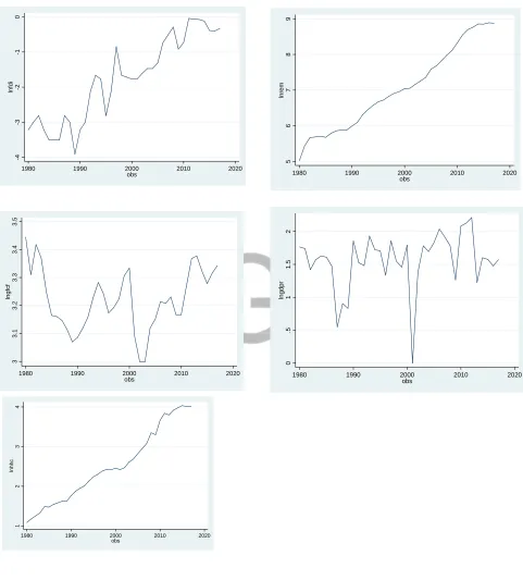
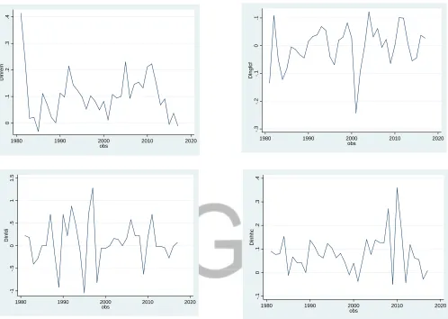
Figure 2 and Figure 3 illustrate the stationary level of the variables. Figure 2 shows the data
series of all variables household consumption (hhc), foreign direct investment (fdi) and gross
fixed capital formation (gfcf)except GDP growth rate are non-stationary at level. In this situation
it is essential to convert the data into stationary. Figure 3 presents the view of stationary of the
5 6 7 8 9 ln re m
1980 1990 2000 2010 2020
obs 1 2 3 4 ln h h c
1980 1990 2000 2010 2020
obs 3 3 .1 3 .2 3 .3 3 .4 3 .5 ln g fc f
1980 1990 2000 2010 2020
obs 0 .5 1 1 .5 2 ln g d p r
1980 1990 2000 2010 2020
obs -4 -3 -2 -1 0 ln fd i
1980 1990 2000 2010 2020
obs
-. 3 -. 2 -. 1 0 .1 D ln g fc f
1980 1990 2000 2010 2020
obs 0 .1 .2 .3 .4 D ln re m
1980 1990 2000 2010 2020
obs -. 1 0 .1 .2 .3 .4 D ln h h c
1980 1990 2000 2010 2020
obs -1 -. 5 0 .5 1 1 .5 D ln fd i
1980 1990 2000 2010 2020
obs
Figure 2 Graphical Illustration of data on First difference
3.1. Unit Root Test
The unit root test is performed using the Augmented Dickey Fuller (ADF) unit root test. This test
is performed to ensure that none of the variables are I (2) too. The results are shown in Table 1.
Table shows all the variables are none stationary at levels and become stationary at first
difference except for gross domestic product growth rate. Gross domestic product growth rate is
stationary at level which means it is integrated of order zero, I (0). This implies that the unit root
Table 3.1. Unit Root Test
variables Level I (0) 1st Difference I (1)
Test Statistic 5% Critical Value Test Statistic 5% Critical Value
lngdpr -4.755 -2.966
lngfcf -2.593 -2.966 -4.921 -2.969
lnrem -0.732 -2.966 -4.894 -2.969
lnhhc 0.052 -2.966 -6.175 -2.969
lnfdi -1.219 -2.966 -6.252 -2.969
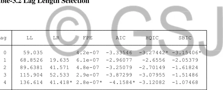
Table 3.2 reports the optimal lag length of four (4) out of a maximum of 4 lag lengths as selected
by four different criteria: Final Prediction Error (FPE), Akaike information criteria (AIC),
Schwarz Information Criterion and Hannan-Quinn Information Criterion.
Table-3.2 Lag Length Selection
*indicates lag order selected by the criterion
3.2 ARDL Bounds Test for Cointegration
Following the unit root test and establishing that none of the variables are I(2), the study examine
the long run relationship among the variables. Starting with gross domestic product growthrate
as the dependent variable, the calculated F-statistics is 28.866. The critical values ranges are I(0)
= 4.914 and I(1)= 7.299 at 1% level of significance. Therefore, comparing the F-statistics with
the critical values, it indicates that F-statistics is greater than the upper critical value at 1% level
of significance. This suggests that the null hypothesis of no cointegration will be rejected Exogenous: _cons
Endogenous: lngdpr Dlngfcf Dlnrem Dlnfdi
4 136.614 41.418* 16 0.000 2.8e-07* -4.1584* -3.12082 -1.07468 3 115.904 52.533 16 0.000 2.9e-07 -3.87299 -3.07955 -1.51486 2 89.6381 41.571 16 0.000 4.8e-07 -3.25079 -2.70149 -1.61824 1 68.8526 19.635 16 0.237 6.1e-07 -2.96077 -2.6556 -2.05379 0 59.035 4.2e-07 -3.33546 -3.27442* -3.15406* lag LL LR df p FPE AIC HQIC SBIC Sample: 1985 - 2017 Number of obs = 33 Selection-order criteria
. varsoc lngdpr Dlngfcf Dlnrem Dlnfdi
Exogenous: _cons
Endogenous: lngdpr Dlngfcf Dlnrem Dlnfdi
4 136.614 41.418* 16 0.000 2.8e-07* -4.1584* -3.12082 -1.07468 3 115.904 52.533 16 0.000 2.9e-07 -3.87299 -3.07955 -1.51486 2 89.6381 41.571 16 0.000 4.8e-07 -3.25079 -2.70149 -1.61824 1 68.8526 19.635 16 0.237 6.1e-07 -2.96077 -2.6556 -2.05379 0 59.035 4.2e-07 -3.33546 -3.27442* -3.15406* lag LL LR df p FPE AIC HQIC SBIC Sample: 1985 - 2017 Number of obs = 33 Selection-order criteria
indicating the existence of long-run relationship between the variables. Nevertheless, since four
of co-integration equations validate the existence of a long run relationship between the
variables, here the study conclude that there is a long run relationship between gross fixed capital
formation, remittance, household consumption and foreign direct investment in Sri Lanka.
Table 3.3 ARDL bound test for Cointegration
ARDL Co-integration test
Lag length F-statistic
ARDL (1,3,4,3,2) 28.866***
Significance level Critical values *
Lower bounds I (0) Upper bounds I (1)
1 percent 4.914 7.299
5 percent 3.286 5.042
10 percent 2.644 4.144
Diagnostic tests
NORMAL SERIAL Heteroskedasticity WHITE
0.3989 (0.1200)
1.984674 (0.9949)
16.09 (0.3079)
11.17 (0.6728)
The long-run coefficients are reported in the output section LR. They represent the equilibrium
effects of the independent variables on the dependent variable. In the presence of cointegration,
they correspond to the negative cointegration coefficients after normalizing the coefficient of the
dependent variable to unity. The latter is not explicitly displayed.
Table 3.4: Long Run coefficients estimated through ARDL approach
Variable Coefficients Standard Error T-statistics Probability
dlngfcf 7.514862 1.189843 6.32 0.000
dlnrem 5.736542 1.555356 3.69 0.002
dlnhhc -2.217659 1.393849 -1.59 0.132
dlnfdi -.2866454 .1500486 -1.91 0.075
The study next involves estimating the long run coefficients and the results are demonstrated in
statistically significant and positively correlated with gross domestin production growth rate in
the long run. Specifically, the coefficient of gross fixed capital formation is 7.514862, which
implies that a 1% increase in gross fixed capital formation leads to 7.514862% increase in gross
domestic production growth. The results are consistent to studies conducted by Bayar (2015) and
Ahmed (2010). The coefficient of remittance is 5.736542, which means that a 1% increase in
remittance results in an increase of about 5.736542% in gross domestin production growth. The
results are consistent to studies conducted by Huseyin and Bayar (2015) Dietmar and Adela
(2017) and Siddique et al (2010). Household consumption and foreign direct investment are not
statistically significant and have a negative effect on gross domestic production growth in long
run.
The negative speed-of-adjustment coefficient is reported in the output section ADJ. It measures
how strongly the dependent variable reacts to a deviation from the equilibrium relationship in
one period or how quickly such an equilibrium distortion is corrected. The short-run coefficients
are reported in the output section SR. They account for short-run fluctuations not due to
Table 3.5 Short run analysis
Dependent Variable = lngdpr (gross domestic production growth rate)
Short Term Results
Variable Coefficients Standard Error T-statistics Probability
gross fixed capital formation dlngfcf
D1. -2.728804 1.050135 -2.60 0.020
LD. -2.094895 .7924327 -2.64 0.018
L2D. -2.411175 .5944936 -4.06 0.001
remittance dlnrem
D1. -4.407966 1.415599 -3.11 0.007
LD. -3.280226 1.099722 -2.98 0.009
L2D. -3.314654 .815624 -4.06 0.001
L3D. -1.604046 .6087015 -2.64 0.019
Household consumption dlnhhc
D1. 3.242746 1.250392 2.59 0.020
LD. 2.08482 .8153963 2.56 0.022
L2D. 1.843952 .423426 4.35 0.001
foreign direct investment dlnfdi
D1. 3.242746 1.250392 2.59 0.020
LD. 2.08482 .8153963 2.56 0.022
ADJ lngdpr
L1. -1.157316 .1244126 -9.30 0.000
R2 0.9710
Adj R-squared 0.9381
Table 3.5 illustrates the short run results and the speed of adjustment coefficient (ADJ). It is
established that the coefficient of the adjustment (-1.157316) is negative and statistically
significant at the 1% level of significance. This indicates that approximately 115% of the
disequilibrium of gross domestic production growth rate shock of the previous year will result in
the adjustment back to the long run rate equilibrium of gross domestic production growth rate
and a statistically significant effect on gross domestic production growth rate except for gross
fixed capital formation and remittance in the short run. Gross fixed capital formation and
remittance have a negative effect on domestic production growth rate but they are statistically
significant.
Results of the diagnostic tests show that the estimated ARDL model and the error-correction
models do not have serial correlation, heteroscedasticity, specification error, and nonnormality at
the 5% significance level. As is evident from Table 3.3, all the 𝑃 values of the diagnostic tests
are greater than 5%, implying that the null hypotheses of no serial correlation, homoscedasticity,
normality, and specification error cannot be rejected at the 5% significance level.
Stability Tests
Finally, this study explored the stability of the long-run trends together with the short-run
movements of the variables. Cumulative sum squares (CUSUMSQ) tests was applied to explore
the stability of the long run which proposed by Borensztein et al. (1998). This same process has
been applied by Pesaran and Pesaran (1997), Mohsen et al. (2002) and Suleiman (2005) to test
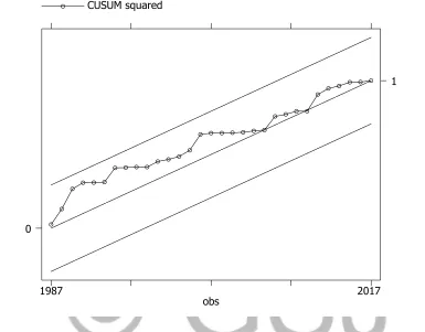
Figure - 1 Cumulative sum squares (CUSUMSQ) tests
Figures 1 plot the CUSUM of squares statistics and CUSUMSQ stays within the critical 5%
bounds that confirms the long-run relationships among variables and thus shows the stability of
coefficient.
CONCLUSION
This study investigated the relationship between gross domestic growth rate, remittance, gross
fixed capital formation, household consumption and foreign direct investment of Sri Lanka
during the period of 1980 to 2017 by employing the ARDL bound test approach. Bound test
suggested that the remittances have the long run negative relationship with economic growth of
Sri Lanka. The model having lag 2 is the best model, because it has no serial correlation, no
heteroskedasticity and residuals are normally distributed. The model is also stable. The model
has getting towards long run equilibrium at the speed of 1.157316. The model has short run
causality from independent variables to dependent variable. Also, it has long run association
among the variables and they move together. The error correction term of this models is highly
CU
SU
M
s
qu
ar
ed
obs CUSUM squared
1987 2017
0
significant and correctly singed. This shows adjustment to long term equilibrium in the dynamic
model. The coefficients of error correction are (-1.157316). This indicates that deviations from
the remittance to economic growth adjust quickly. Dang Tung (2015), Shapan and Zhang (2016)
findings are supported the coefficient on the error correction term, ECM (–1), is significant and
negative at the 1 percent level, which permits the existence of the long-run relationship among
the variables in this model found by the F-test.
References
Ahmed, M. S., (2010). Migrant Workers Remittance and Economic Growth: Evidence from
Bangladesh. ASA University Review, Vol. 4 No. 1 (January-June), pp. 1-13;
Bayar, Y., (2015). Impact of Remittances on the Economic Growth in the Transitional
Economies of the European Union. Economic Insights – Trends and Challenges, 4(…) Vol.
IV(LXVII) No. 3, 1-10. http://www.upg-bulletin-se.ro/archive/2015-3/1.Bayar.pdf
Dietmar Meyera and Adela Sherab, 2017. The impact of remittances on economic growth: An
econometric model EconomiA 18 147–155
Dang Tung 2015 Remittances and Economic Growth in Vietnam: An ARDL Bounds Testing
Approach, Review of Business and Economics Studies, 3(1)
Gyan Pradhana, Mukti Upadhyayb and Kamal Upadhyayac, 2008. Remittances and economic
growth in developing countries, The European Journal of Development Research 20(3), 497–506
Huseyin Karamelikli and Yılmaz Bayar, 2015. Remittances and Economic Growth in Turkey
ECOFORUM 4, 2 (7)
Mesbah Fathy Sharaf, 2014. The Remittances-Output Nexus: Empirical Evidence from Egypt
Hindawi Publishing Corporation, Economics Research International.
Nsiah Christain and Bichaka Fayissa, 2008. “The impact of Remittances on economic growth
and Development in Africa,” Working papers 200802, Middle Tennessee State University,
Department of Economics and Finance.
Rahman, M. (2009). Contribution of Exports, FDI, and Expatriates’ Remittances to Real GDP of
Bangladesh, India, Pakistan and Sri Lanka. Southwestern Economic Review, 36, 141-153
Rahman, M., Mustafa, M., Islam, M., and Guru-Gharana, K. K., (2006). Growth and
Employment Empirics of Bangladesh. Journal of Developing Areas, 40(1), 99-114.
Shapan Chandra Majumder and Zhang Donghui, 2016. Relationship between Remittance and
Economic Growth in Bangladesh: An Autoregressive Distributed Lag Model (ARDL) European
Researcher 104(3),156-167 www.erjournal.ru
Siddique, A., Selvanathan, E. A., and Selvanathan, S. (2010). Remittances and Economic
Growth: Empirical Evidence from Bangladesh, India and Sri Lanka, Discussion Study,