A Model of Self-Avoiding Random Walks for Searching Complex Networks

A Model of Self-Avoiding Random Walks for Searching Complex

Networks

V´ıctor M. L´opez Mill´an1_{, Vicent Cholvi}2_{, Luis L´opez}3_{, and Antonio Fern´andez Anta}4

1_{Universidad CEU San Pablo, Madrid, Spain (Assistant Professor)}

2_{Universitat Jaume I, Castell´on, Spain (Associate Professor)}

3_{Universidad Rey Juan Carlos, Madrid, Spain (Assistant Professor)}

4_{Institute IMDEA Networks, Madrid, Spain (Full Professor)}∗

May 28, 2011

Abstract

are very close to simulation results, and allow us to draw conclusions about the applicability of SAWs to network search.

Keywords: self-avoiding random walk, random walk, network search, resource location, one-hop

replication, average search length

1

Introduction

Arandom walk in a network is a simple routing mechanism that chooses the next node in the route

uniformly at random among the neighbors of the current node. Although naive, this mechanism

proves useful especially in situations where there is no complete knowledge about the network or

where the network changes frequently, like the Internet, the WWW, peer-to-peer (P2P) networks

and wireless ad-hoc networks. Some of the advantages derived from its simplicity are that it

needs little processing power in the nodes and that it requires only local information, avoiding the

bandwidth overhead produced by the exchange of routing information among nodes. Applications

of random walks include routing, searching, network sampling, network construction and network characterization [2, 3, 8, 11, 14, 16, 17, 22, 23, 25, 26, 27, 35, 36, 40].

Random walks on graphs have been extensively analyzed in Mathematics [19, 24, 31], where they

are typically modelled as Markov chains, leading to many interesting results that include bounds

on the cover time [4, 7, 15, 20, 30, 42] (i.e., the number of steps to visit all, or a fraction of, the

nodes in the graph), and bounds on theaccess time [9, 33] (the expected number of steps to reach

node j starting from node i). These results are frequently based on the spectral properties of the

adjacency matrix of the graph and of the transition matrix of the random walk. Random walks

have also received much attention from the Physics community, since they reflect the dynamics of

many natural systems including protein interactions, polymer chains, communication networks, and social networks.

The basic behavior of a random walk can be modified in a number of ways to optimize its

performance metrics on networks. Costa and Travieso [13] study the network coverage of three

types of random walks: traditional, preferential to untracked links, and preferential to unvisited

nodes. They find that the latter is the best strategy in covering the network nodes, in both random

random walk variations: no-back (NB), no-triangle-loop (NTL), no-quadrangle-loop (NQL),

self-avoiding (SA) and high-degree-preferential self-self-avoiding (PSA). He finds that all algorithms achieve

similar performance in random networks, while the self-avoiding walk outperforms the others in

scale-free networks and small-world networks. Both results suggest that a random walk that tries to not revisit nodes is an interesting alternative to pure random walks for network search. Our

work focuses on using this type of walk for searching for resources in a network. More concretely,

we define a walk that chooses the next node to be visited uniformly at random among the unvisited

neighbors of the current node. If no unvisited neighbor exists, the next node is chosen uniformly at

random among all the neighbors of the current node. The walk proceeds until it finds the resource

searched for. We will refer to such a walk as a self-avoiding walk (SAW) in this paper.

Our model of SAW is in fact akin to the true SAW defined in [5] at short times, becoming a

simple random walk at long times. The true (or myopic) SAW is defined as the stochastic process

which chooses the next node to be visited among the neighbors of the current node with probability

proportional to a negative exponential of the number of times visited. Our definition of SAW differs

from this one in that the next node is chosen uniformly at random among the unvisited neighbors

or, if none, among all neighbors, regardless of how often they have been visited in the past. This

means that our SAW model loses its self-avoiding properties at long times, while the true SAW

keeps them at all times.

The analysis of the self-avoiding walk with analytical tools is hard since, unlike the pure random

walk, it cannot be modelled as a Markovian stochastic process. Therefore, many questions on

SAWs have not yet been answered in an analytical manner. In addition, using analytical results in some real scenarios is impractical when the adjacency matrix of the network is too large or simply

unknown. In Mathematics, a SAW is defined as a random walk restricted not to intersect with

itself. Note that this definition is more restrictive than the one established above in networks, since

such a walk never revisits a node, having therefore finite length always. We will refer to this type

of walk as strict SAW, to avoid confusion with the SAW we are interested in to search complex

networks. Available results on strict SAWs are compiled in [38]. This work also includes results on a

less restrictive version called theweakly self-avoiding walk, in which intersections are not disallowed

visited nodes.

Works from the mathematical point of view like the ones referenced and others [21, 28, 39, 38],

study SAWs in d-dimensional lattices (Zd_{). Results include the behavior of the number of SAWs}

with n-steps in the lattice and of the mean-square displacement (the average distance between the

end and the origin of a walk). In complex networks, questions have been addressed mostly through

empirical approaches. The previously cited works by Costa and Travieso [13], and Yang [41] use

numerical simulations. Mean access times in lattices with embedded scale-free networks providing

long-range shortcuts have been obtained in [10]. In [18], strict SAWs are studied in scale-free

networks, obtaining approximate analytical expressions for the mean number of SAWs starting from

a generic node, and for the average maximum length of such walks over statistically independent

networks. Simulation results support their approximate analytical calculations.

1.1 Contributions

This paper studies SAW as a search mechanism in communication networks. Our main contribution

is an analytical model that estimates the average search performance of SAWs in complex networks

with or without one-hop replication, and where a number of instances of the resource sought are

present. In aone-hop replication network, a node knows about the resources held by its neighbors.

Therefore, to find a resource in such a network it suffices to visit a node that holds it or any of

its neighbors, whereas the walk must visit a node that holds the resource if one-hop replication

is not available. One-hop replication is an interesting feature in a communication network, since

it contributes to reducing search lengths at limited cost. It has been included as part of search

mechanisms in P2P networks [11, 12, 29, 35].

In particular, our model estimates the network coverage attained at each hop of the walk and

uses this to estimate the average search length. Although our definition of a SAW coincides with

those of a walk preferential to unvisited nodes in [13] and of aself-avoiding (SA) walk in [41], our

work differs from them in that we propose an analytical model to predict network coverage and search performance, whereas their evaluations are only based on simulation results. In addition, [13]

evaluates network coverage (not network search).

We follow the approach that Rodero-Merino et al. [35] apply to “pure” random walks in

functions of their values at the previous hop. The model is based on networks determined only by

their size and degree distribution, with no particular topology assumed. Therefore, it is, as the one

in [35], a mean-field model.

The accuracy of the model predictions has been assessed using simulations. Three types of random networks have been considered for our experiments: (1) regular networks, where the degree

is constant for all nodes, (2) Erd˝os-R´enyi (ER) networks, also called random networks, where there

is a fixed probability that a node is linked to any other node in the network, and (3) scale-free

networks, where the degree distribution obeys a power-law behavior in the node degree. Scale-free

networks are of special interest since many real communication networks exhibit power-law degree

distributions, including the Internet, the WWW, and P2P networks [1, 6, 34, 37].

The networks in the experiments are built using the random mechanism proposed by Newman et

al. [32] for networks with arbitrary degree distributions. For each network type, results are averaged over all searches performed in a network, and then over all the networks built. We have found that

the model predictions are good approximations of the values obtained this way. Therefore, the model

proposed is useful to predict average SAW search performance in large networks built randomly, as

is the case, for example, of unstructured P2P resource-sharing systems.

Finally, we contribute some useful conclusions from the comparison of the performance of a SAW

and a pure random walk for searching networks. As an example, it has been found, in accordance

with [13, 41], that the SAW outperforms the pure random walk by obtaining shorter searches on

the average, especially in scale-free networks. However, we have noticed that the performance gain

is large in networks without hop replication, but it is sensibly smaller for networks with one-hop replication. This is a consequence of the observed fact that, in one-one-hop replication networks,

an average random walk covers nodes (i.e., visited nodes and neighbors of them) almost as fast

as an average SAW. This means that the effect on average search length of one-hop replication is

nearly equivalent to that of trying not to revisit nodes. This observation suggests that SAWs are an

interesting alternative to pure random walks for searching networks without one-hop replication,

which avoids the overhead of updating information about the neighbors’ resources.

Summarizing, our work provides the following contributions:

SAW in randomly built networks characterized by their size and degree distribution. The

model takes into account the existence of one-hop replication and the multiplicity of instances

of the resource searched for.

• An extension of the previous RW model proposed in [35] to support networks without one-hop

replication and with more than one instance of the resource searched for.

• A study of the search performance of SAW in networks with one-hop replication. Simulations

are used to validate the model predictions. Results have been compared with those of random

walks in the same type of network and with search performance of RW and SAW in networks

without one-hop replication.

• The observation that SAW achieves large reductions in the average search length with respect

to RW in networks without one-hop replication, while reductions are moderate in networks

with one-hop replication. These reductions decrease as the average degree of the network

grows, except for scale-free networks without one-hop replication, where the reductions

in-crease with the average degree.

The rest of the paper is organized as follows. Section 2 presents our analytical model for the

estimation of network coverage and search lengths of self-avoiding walks. Section 3 analyzes the

performance of the SAW in comparison with that of a pure random walk in networks with and

without one-hop replication. Simulation results are provided to validate the model derived in the

previous section. Finally, Section 4 states our conclusions and outlines some future work lines.

2

The Analytical Model

2.1 Definitions and Assumptions

Let G(V, E) be an undirected graph representing a communication network where V is the set of

its nodes and E is the set of its links. The network is assumed to be connected (i.e., there is some

path connecting every pair of different nodes in the network). The network is characterized solely

by the number of nodes (N) and by its degree distribution pk, where pk is the probability that a

network (i.e.,!_knk=N), thenpk =nk/N. Anattachment point is a point in a node where one of

the two ends of a link is attached. Therefore, each node has a number of attachment points equal

to its degree, and the total number of attachment points in the network is S =!_kknk, which is

also twice the total number of links in the network. Auto-links (links connecting a node to itself) and multilinks (more than one link between two nodes) are disallowed [35, 18].

The proposed model does not take into account the topology ofGto characterize networks. This

means that it is in fact amean-field model, whose accuracy is checked using simulation experiments.

Empirical results for sets of regular, ER and scale-free networks built randomly show that model

predictions are good approximations for those classes of networks. However, we believe it is possible

to find classes of networks for which the structure is more important than the degree distribution,

and for which the mean-field model predictions are not good approximations of real values.

The fact that the model does not consider network topology is reflected in the formalism in that

it is assumed that given any attachment point of an arbitrary node i, the link departing from it

can take us to any other attachment point (of a nodej _!=i) in the network with equal probability.

This condition, used also in the mean-field study in [35], is true for networks built with the random

mechanism proposed by Newman [32].

We define a self-avoiding walk (SAW) as a random walk governed by the rules: (R1) if all

neighbors of the current node have been already visited, choose the next node uniformly at random

among all neighbors (including the one the walk came from), and (R2) if there is at least one

unvisited neighbor of the current node, choose the next node uniformly at random among the

unvisited neighbors.

We assume that the walk will search the network for a particular resource, starting at a node

chosen uniformly at random from all network nodes (at hop h = 0). There are R >0 instances

of the resource sought. This allows us to model scenarios with multiplicity of resource instances

such as peer-to-peer (P2P) networks, where several peers contain the same file [17]. We assume

that these instances are held by (different) nodes chosen uniformly at random. In networks without

one-hop replication, the search will finish when the walk visits any node holding an instance of the

resource. In networks with one-hop replication, visiting a neighbor of any node holding the resource

as the average number of hops it takes to find an instance of the resource sought. This magnitude

depends on the number of different nodes that the walk has visited (denoted V(h)) or covered

(denotedC(h)) up to and including hoph. In turn,V(h) andC(h) depend on a number of auxiliary

magnitudes that capture the behavior of the SAW. These magnitudes are defined in Table 1 and their expressions are derived in the next paragraphs.

2.2 Visited nodes

We start by estimatingPk

w(h), the probability of visiting any nodejof degreekat hoph, given that

the walk is currently at some nodei. Two different cases need to be considered: (1) all neighbors of

ihave already been visited, and (2) at least one neighbor ofihas not been visited yet, corresponding

to rules R1 andR2 of the SAW, respectively.

• Case 1: This probability is the ratio of “positive” attachment points and possible attachment

points. We consider attachment points belonging to nodes of degree k to be positive and all

attachment points in the network to be possible1_{. The probability of visiting any node j of}

degree kat hop h, conditioned on the fact that all neighbors of ihave already been visited is

then:

P_wk_,anv = knk

S =

knk

!

jjnj =

kpk

!

jjpj =

kpk

k , for h >0,

P_wk_,anv(0) = pk. (1)

Here, we are using our assumption that a given attachment point of i can take us to any

attachment point in the network with equal probability. We are also taking into account the

fact that the attachment point ofiwill be chosen uniformly at random for hoph, asR1 states.

Note that this probability is not a function of the hoph (except forh= 0), since the behavior

is that of a random walk, whose next state depends only on the current state and not on the

1_{To be fully precise, the attachment points of ishould not be considered either as possible or positive (in case}

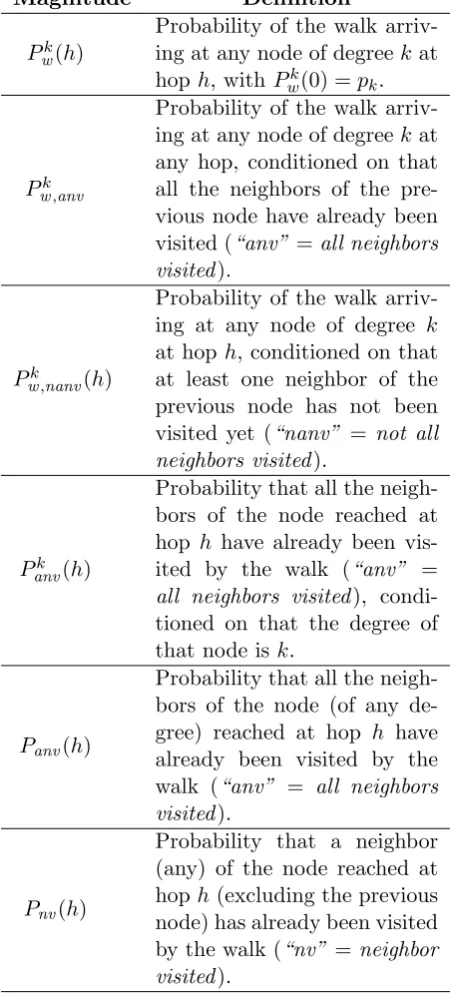
Magnitude Definition

P_wk(h)

Probability of the walk

arriv-ing at any node of degreekat

hop h, with Pk

w(0) =pk.

Pk w,anv

Probability of the walk

arriv-ing at any node of degreekat

any hop, conditioned on that all the neighbors of the pre-vious node have already been

visited (“anv” =all neighbors

visited).

P_wk_,nanv(h)

Probability of the walk

arriv-ing at any node of degree k

at hop h, conditioned on that

at least one neighbor of the previous node has not been

visited yet (“nanv” = not all

neighbors visited).

P_anvk (h)

Probability that all the neigh-bors of the node reached at

hop h have already been

vis-ited by the walk (“anv” =

all neighbors visited), condi-tioned on that the degree of

that node is k.

Panv(h)

Probability that all the neigh-bors of the node (of any

de-gree) reached at hop h have

already been visited by the

walk (“anv” = all neighbors

visited).

Pnv(h)

Probability that a neighbor (any) of the node reached at

hop h(excluding the previous

node) has already been visited

by the walk (“nv” =neighbor

visited).

past history of the walk. For h = 0, the node is chosen uniformly at random among all the

nodes in the network, so the probability of reaching a node of degree kis pk.

• Case 2: Positive cases are now only those attachment points belonging to non-visited nodes of

degreek. Similarly, possible attachment points are now only those belonging to all non-visited

nodes. Let us denote byVk_{(h) the average number ofdifferent nodes of each degreekvisited}

by the walk up to and including hop h. We obtain the number of non-visited nodes from the

number of visited nodes at the previous hop (Vk_{(h−1)). Thus, the probability of visiting any}

node j of degree k at hoph, conditioned on the fact that not all neighbors ofihave already

been visited is:

P_wk_,nanv(h) = k(nk−V

k_(h−1))

S₋"

j

jVj(h₋1) =

k(pk−V k_(h−1)

N )

k₋"

j

jV

j_(h−1)

N

, for h >0,

P_wk_,nanv(0) = pk. (2)

This probability does depend on the hoph since the number of visited nodes increases as the

walk proceeds through the network.

Using Equations (1) and (2), and taking into account thatPanv(h−1) and (1−Panv(h−1)) are

the probabilities that the SAW follows R1 and R2 at hoph, respectively, we have that Pwk(h) can

now be obtained as:

P_wk(h) =P_wk_,anv·Panv(h−1) + Pwk,nanv(h)·(1−Panv(h−1)), for h >0,

P_wk(0) = pk. (3)

On the other hand, Panv(h) depends on the number of neighbors of the node reached at hop

h (i.e., its degree), and can be obtained from the probabilities that all neighbors of the node have

already been visited conditioned on the fact that the degree of that node is k:

Panv(h) =

"

k

At this point, we note that:

P_anvk (h) = (Pnv(h))k−1. (5)

The node from which the walk came from is excluded from the calculation (thus the exponentk₋1),

since it is certain that this node has already been visited. We are implicitly assuming here that each

of the neighbors of the node are visited or not independently from the others. This approximation

has been shown to be accurate in the types of network we consider [35].

The probability of a neighbor having been visited depends in turn on the degree of that

neigh-bor, since nodes with higher degree have higher chance of being visited. This probability is thus

calculated as:

Pnv(h) =

"

k

P_wk_,anvV

k_(h−2)

nk

, for h >1,

Pnv(0) = 0,

Pnv(1) = 0. (6)

P_wk_,anv plays here the role of the probability that the neighbor is of degreek (the probability of

visiting a node of degree k from the current node when it is chosen uniformly at random), while

the fraction within the summation gives the probability of a neighbor of degree k being already

visited as the ratio of positive nodes and possible nodes. Here, Vk(h−2) is used instead of Vk(h)

to exclude the node reached at hoph (in case its degree isk) and the node the walk came from (in

case its degree is k). The latter is certain to have been visited already as stated above, and thus

does not participate in the calculation of Pk

anv(h).

Vk(h) can now be estimated using the following recursive expression:

Vk(h) = Vk(h−1) +P_wk_,nanv(h)·(1−Panv(h−1)), for h >0,

Vk(0) = pk, (7)

since a new node of degree kis visited at hop hwith probabilityPk

w,nanv(h) given that the routing

number of different nodes visited by the walk up to and including hop h is then:

V(h) ="

k

Vk(h). (8)

2.3 Covered Nodes

This magnitude estimates the average number of nodes covered by the walk up to and including

hop h, denoted byC(h). A node iscovered by the SAW when the walk visits that node or any one

of its neighbors. The number of nodes covered by the walk allows the estimation of average search

length in one-hop replication networks in the last step of our analysis, since to find a resource in

such a network it suffices to cover (not to visit) the node that holds it.

We first estimateCk_{(h), the average number of different nodes of degreek covered by the walk}

up to and including hoph, in order to obtain C(h).

For networks with a given degree distribution, the average number of nodes of degreek that a

walk covers at each hop clearly depends on the routing algorithm used. An expression forC(h) was

obtained in [35] for a pure random walk in the same types of network as those considered in our

work. It is expressed in terms of the average number of visited nodes of each degree (Vk(h)) and

the degree distribution of the network, where Vk(h) contains the effect of the routing algorithm.

Therefore, that expression is still valid if we change the random walk into a SAW provided that

we use the expressions for Vk_{(h) derived above for the SAW. Thus, the average number of covered}

nodes of degree kcan be written as:

Ck(h) = Ck(h₋1) +     

k&nk−Ck(h−1)

'

S₋"

j

j_·Vj(h₋1)     ×

"

j

&

Vj(h)₋Vj(h₋1)'(j₋1), for h >0,

Ck(0) = Vk(0) +kP_wk_,anv. (9)

Finally, the average number of covered nodes is obtained as:

C(h) ="

k

2.4 Search Length

The average search length is obtained from the probability of finishing the search at hoph(Pf in(h)),

that is in turn obtained from the probability of being successful in finding the resource at hop h

(Psuc(h)):

h=

∞

"

h=0

h·Pf in(h), (11)

where

Pf in(h) = Psuc(h) h₊−1

i=0

(1−Psuc(i)), for h >0,

Pf in(0) =

R

N. (12)

Recall that there are R instances of the resource, placed in different nodes. Now, Psuc(h) depends

on whether or not the networks considered are one-hop replication networks. For networks without

replication, Psuc(h) can be estimated as the relation between the number of new nodes visited at

hop hand the number of nodes that are still unvisited at that hop, taking into account the number

of resource instances:

Psuc(h) = R

V(h)₋V(h₋1)

N₋V(h₋1) , for h >0,

Psuc(0) = R

N. (13)

For one-hop replication networks, Psuc(h) can be similarly estimated as the relation between the

number of new nodes covered at hop h and the number of nodes that are still uncovered at that

hop:

Psuc(h) = R

C(h)₋C(h₋1)

N−C(h−1) , for h >0,

Psuc(0) =

R

N. (14)

From Equations (11), (13) and (14) we can finally write the average search length in networks

hnr = ∞

"

h=1

h ,

RV(h)−V(h−1) N₋V(h₋1) ·

-1₋RV(0)

N .

·

h₊−1

i=1

-1−RV(i)−V(i−1) N₋V(i₋1)

./

, (15)

and

h1hr = ∞

"

h=1

h ,

RC(h)−C(h−1) N₋C(h₋1) ·

-1−RC(0)

N .

·

h₊−1

i=1

-1−RC(i)−C(i−1) N₋C(i₋1)

./

. (16)

Note that both hnr and h1hr depend only on the network parameters, namelyN,pk and R.

3

Performance Evaluation

In this section, we assess the accuracy of the SAW model comparing its predictions against

simula-tion results. At the same time, we compare the performance of SAWs and pure random walks (RW) for searching complex networks. Experiments have been performed for three types of randomly

built networks: regular networks, Erd˝os-R´enyi networks (referred to as ER random networks or

just random networks) and scale-free (power-law) networks. Network size has been set toN = 104

nodes in the base experiment, and three average degrees have been used (k= 10,20,30) to observe

the effect of network connectivity.

ER random networks with degree averages k = 10,20,30 have been obtained with link

prob-abilities p = 0.001,0.002 and 0.003, respectively. Scale-free networks follow a power-law degree

distribution (p(k)_∝k−γ_{) withγ values of 2.7030, 1.9958 and 1.781, adjusted to obtain feasible}

net-works with average degreesk= 10,20,30, respectively. For this type of network, a minimum degree

of 5 has been set to avoid disconnected networks due to the high numbers of low degree nodes. The

degree distributions thus obtained are then used to feed the SAW and random walk models2_{, and to}

construct the networks for simulations using Newman’s method. This method guarantees that each

2_{For the pure random walk, we have used the analytical model in one-hop replication networks proposed in [35],}

attachment point is linked to any other attachment point in the network with equal probability,

which is an assumption of the model as stated in Section 2.1.

To be able to fairly compare the predictions of the mean-field models with the experimental

results, simulations have been run for a representative number of different networks (102_{) with that}

degree distribution, and for a representative number of walks (103_{) for each of those networks,}

resulting in a total of 105 _{simulation runs for each experiment. Magnitudes are measured for each}

walk and values averaged over all walks in that network to obtain the network average. Network

averages are in turn averaged over all networks to obtain the final average values to be compared

with those estimated by the models. Variations of network averages compared to final average

values have also been studied, finding that average values for individual networks are close to final

network average values. Results for minimum, average, and maximum values, along with the typical

deviation, are shown for the average search length later in this section.

We begin by showing results for two auxiliary magnitudes: the probability that all neighbors of

a node have already been visited and the probability of visiting a node of degree k. These results

will be shown for ER random networks only, as an illustration of the behavior of the SAW. Next,

we show results for the average number of nodes visited (V(h)) and covered (C(h)) by the walks,

which are determined by the previous probabilities. Finally, results for average search lengths (h)

are shown.

3.1 Auxiliary magnitudes

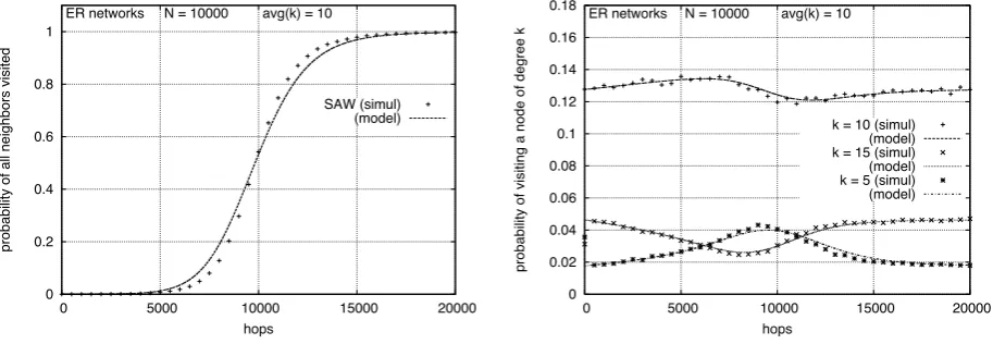
Figure 1(a) shows Panv(h), the probability that all the neighbors of a node (of any degree) reached

at hophhave already been visited, in ER random networks withk= 10. It is an interesting starting

point, since this probability can also be interpreted as the probability that the SAW actually succeeds

in avoiding already visited nodes, or else it falls back to the RW behavior.

This figure clearly shows three different regions or phases, which correspond to different

behav-iors of the SAW. The probability that all neighbors of the node have already been visited is very low up to around 7500 hops, which is 75% the size of the network. Therefore, the SAW will visit a

new node in every hop with high probability in this region. Then, the probability that all neighbors

0 0.2 0.4 0.6 0.8 1

0 5000 10000 15000 20000

probability of all neighbors visited

hops

SAW (simul) (model) ER networks N = 10000 avg(k) = 10

(a) Probability of all neighbors visited (Panv(h)).

0 0.02 0.04 0.06 0.08 0.1 0.12 0.14 0.16 0.18

0 5000 10000 15000 20000

probability of visiting a node of degree k

hops

k = 10 (simul) (model) k = 15 (simul) (model) k = 5 (simul) (model) ER networks N = 10000 avg(k) = 10

(b) Probability of visiting a node of degreek(Pk w(h)).

Figure 1: Auxiliary magnitudes of the SAW model in ER random networks withk= 10.

For numbers of hops greater than 12500, the probability grows asymptotically to 1. In this region the SAW behaves very much like a RW, since it is almost certain that all neighbors of the nodes

reached have already been visited.

This figure also shows that the model predicts results with a reasonable accuracy. The more

significant deviations between model and simulation results occur in the central region of the graph

(transition phase). For smaller number of hops, the model is pessimistic, that is, it predicts higher

probabilities that all neighbors are visited than the simulation does. This is inverted for greater

number of hops. This will yield pessimistic estimations of the average number of visited and

covered nodes, as will be shown in later subsections. Therefore, the model presented in Section 2 is

a conservative model of the real SAW behavior.

Figure 1(b) showsP_wk(h), the probability of visiting a node of degreekat hoph. This magnitude

is interesting because it shows, like the previous one, the different phases of the algorithm. In

addition, P_wk(h) is the base to estimate the average number of visited and covered nodes, which in

turn are used to estimate the average search length. Curves are presented for three representative

degrees: the average degree (k=k= 10), a degree above the average (k= 15), and a degree below

the average (k= 5). The first thing to note about this graph is that the probabilities for each degree

start (low h) and finish (high h) at the same values. Indeed, when very few nodes are visited, the

Likewise, when almost all nodes have been visited, the probability of visiting a node of some degree

is very similar to that of the RW, since the next hop is chosen uniformly at random among the

(already visited) neighbors of the node. The probability of arriving at a node of degree k at any

hop (P_Ak) in the RW model [35] is the same as the probability of visiting a node of degree kat any

hop if all the neighbors of the current node have already been visited (P_wk_,anv) in the SAW model.

Recall from Subsection 2.2 that this probability is not a function of h, since RW is a memory-less

algorithm. Therefore, in the SAW model P_wk(h) starts at P_wk_,anv = kpk

k for low h and tends to the

same value for high h.

In the first section of the graph (up to about 7500 hops), the SAW visits a new node at each hop

with high probability. Since nodes with higher degrees are visited faster, the probability of visiting

more new nodes of those degrees decrease as h increases. This effect can be seen in Figure 1(b) in

the curve fork= 15. Nodes with lower degrees are visited more slowly, so the probability of visiting

more new nodes of those degrees increases with h. This effect can also be seen in curves for k= 5

and k= 10.

In the second region of the graph (between 7500 and 12500 hops), the transition phase in

Figure 1(a), the probability that all neighbors have been already visited grows rapidly. This will

make the probability of reaching nodes of higher degrees grow to recover the level of P_wk_,anv in the

third region of the graph (h > 12500). On the other hand, the probability of reaching nodes of

lower degrees falls again to the level ofPk

w,anv.

3.2 Visited Nodes

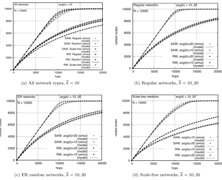
Figure 2(a) shows the average number of visited nodes as a function of the number of hops taken by

the walk (V(h)) for the three types of networks withk= 10. As expected, curves for RW grow more

slowly than curves for SAW, since the latter ones try to avoid revisiting nodes thus visiting new

nodes faster than the former ones. In fact, we notice that SAW achieves a straight line with slope 1

in the first phase of the algorithm, that is, it visits a new node at each hop with a high probability up to a number of hops about 75% of the network size. From then on, new nodes are visited more

slowly in the second phase until the whole network is covered in the third phase. The graph also

0 2000 4000 6000 8000 10000

0 5000 10000 15000 20000

visited nodes

hops

SAW, Regular (simul) (model) SAW, Random (simul) (model) SAW, Scale-free (simul) (model) RW, Regular (simul) (model) RW, Random (simul) (model) RW, Scale-free (simul) (model) All networks

N = 10000

avg(k) = 10

(a) All network types,k= 10

0 2000 4000 6000 8000 10000

0 5000 10000 15000 20000

visited nodes

hops

SAW, avg(k)=20 (simul) (model) SAW, avg(k)=10 (simul) (model) RW, avg(k)=20 (simul) (model) RW, avg(k)=10 (simul) (model) Regular networks

N = 10000

avg(k) = 10, 20

(b) Regular networks,k= 10,20

0 2000 4000 6000 8000 10000

0 5000 10000 15000 20000

visited nodes

hops

SAW, avg(k)=20 (simul) (model) SAW, avg(k)=10 (simul) (model) RW, avg(k)=20 (simul) (model) RW, avg(k)=10 (simul) (model) ER networks

N = 10000

avg(k) = 10, 20

(c) ER random networks,k= 10,20

0 2000 4000 6000 8000 10000

0 5000 10000 15000 20000

visited nodes

hops

SAW, avg(k)=10 (simul) (model) SAW, avg(k)=20 (simul) (model) RW, avg(k)=10 (simul) (model) RW, avg(k)=20 (simul) (model) Scale-free networks

N = 10000

avg(k) = 10, 20

(d) Scale-free networks,k= 10,20

Both SAW and RW curves are higher for regular networks. Curves for ER random networks

are slightly lower and curves for scale-free networks are still farther down. This is an effect of the

different degree distributions of the three types of networks. In regular networks, all nodes are

visited with the same probability, since all of them have the same degree. In random and scale-free networks a number of different degrees are present in the network. Nodes with smaller degrees are

visited with smaller probability than nodes with larger degrees. It is harder for both SAW and

RW to visit nodes with small degrees, resulting in a higher number of revisited nodes and thus in

a slower rate of visiting new nodes. This effect is greater in scale-free networks due to the shape

of power-law distributions: a large number of small degree nodes and a few nodes with a very high

degree (the long tail of the distribution).

Now, we compare the average number of visited nodes in networks with average degreesk= 10

and k = 20 in Figures 2(b) to 2(d). For regular and ER random networks, curves for k = 20 are

always higher than those for k= 10 for both SAW and RW. Since nodes in higher average degree

networks tend to have higher degrees, it is easier to visit new nodes either randomly (RW) or trying

to avoid already visited nodes (SAW), and thus the faster rate of visiting new nodes. However,

the effect is reversed for scale-free networks: curves for k = 20 are lower than those for k = 10.

This can be explained again by the shape of the power-law degree distribution. A higher average

degree network has more very high degree nodes than a lower average degree network. Therefore,

walks keep visiting these nodes with higher probability, making it more difficult to visit low degree

nodes. It can also be seen that the difference is larger for RW than for SAW, since the latter tries

to avoid high degree nodes once they have been visited for the first time, increasing the probability of visiting new nodes.

To further investigate this behavior in the case of SAW, we have checked the probability that all

neighbors of a node have been already visited, since this is also the probability that the next node

will not be a new one. In networks with higher average degree, this probability is indeed higher up

to a number of hops close to the network size. This accounts for the growing divergence between

curves for k= 10 andk= 20 in Figure 2(d). For subsequent hops, the probability of all neighbors

being visited is higher in networks with lower average degree, explaining the convergence of the

been checked to be opposite to that of scale-free networks, consistent with the observed opposite

behavior of the number of visited nodes.

3.3 Covered Nodes

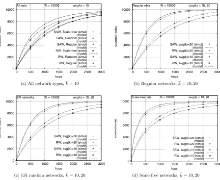
Figure 3(a) shows the average number of covered nodes as a function of the number of hops taken

by the walk (C(h)) for networks of the three types with k = 10. Although SAW always achieves

better rates than RW as expected, the difference here is much smaller than for the average number

of visited nodes (Figure 2(a)). Although RW visits fewer new nodes than SAW, it covers almost

the same number of nodes; more work needs to be done to find out why this is so. This effect reduces the difference in the performance of both algorithms when applied to searching networks

with one-hop replication, as will be shown later in this section.

Figures 3(b) to 3(d) compare the average number of covered nodes in networks with average

degrees k = 10 and k = 20. In regular and ER random networks, curves for k = 20 are higher

than those for k = 10, the same as observed for the average number of visited nodes in

Fig-ures 2(b) and 2(c). In scale-free networks, the curve fork= 20 is also higher than that fork= 10,

in contrast with what was observed for the average number of visited nodes (Figure 2(d)). Although

visiting new nodes in scale-free networks is harder for those with higher average degree, it is easier to cover them because with high probability they are neighbors of the (more numerous) high degree

nodes.

3.4 Search Length

This section shows results for the average search length (h) achieved by SAW and RW in the three

types of networks, with and without one-hop replication. Recall from the definition of the model

(Section 2.4) that h is obtained from the average number of visited nodes (V(h)) for networks

without one-hop replication, while it is obtained from the average number of covered nodes (C(h))

for networks with one-hop replication. We begin by comparing results for a single instance of the

resource in the three types of networks. Then, we study the dependency of h on the number of

instances of the resource in Section 3.5.

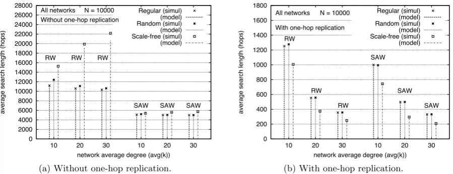
Figure 4 shows the average search length for SAW and RW in the three types of networks, with

0 2000 4000 6000 8000 10000

0 500 1000 1500 2000 2500 3000

covered nodes

hops

SAW, Scale-free (simul) (model) SAW, Random (simul) (model) SAW, Regular (simul) (model) RW, Scale-free (simul) (model) RW, Random (simul) (model) RW, Regular (simul) (model) All nets N = 10000 avg(k) = 10

(a) All network types,k= 10

0 2000 4000 6000 8000 10000

0 500 1000 1500 2000 2500 3000

covered nodes

hops

SAW, avg(k)=20 (simul) (model) RW, avg(k)=20 (simul) (model) SAW, avg(k)=10 (simul) (model) RW, avg(k)=10 (simul) (model)

Regular nets N = 10000 avg(k) = 10, 20

(b) Regular networks,k= 10,20

0 2000 4000 6000 8000 10000

0 500 1000 1500 2000 2500 3000

covered nodes

hops

SAW, avg(k)=20 (simul) (model) RW, avg(k)=20 (simul) (model) SAW, avg(k)=10 (simul) (model) RW, avg(k)=10 (simul) (model)

ER networks N = 10000 avg(k) = 10, 20

(c) ER random networks,k= 10,20

0 2000 4000 6000 8000 10000

0 500 1000 1500 2000 2500 3000

covered nodes

hops

SAW, avg(k)=20 (simul) (model) RW, avg(k)=20 (simul) (model) SAW, avg(k)=10 (simul) (model) RW, avg(k)=10 (simul) (model) Scale-free nets N = 10000 avg(k) = 10, 20

(d) Scale-free networks,k= 10,20

0 2000 4000 6000 8000 10000 12000 14000 16000 18000 20000 22000 24000 26000 28000

10 20 30 10 20 30

average search length (hops)

network average degree (avg(k)) Regular (simul) (model) Random (simul) (model) Scale-free (simul) (model)

All networks N = 10000

Without one-hop replication

RW RW RW

SAW SAW SAW

(a) Without one-hop replication.

0 200 400 600 800 1000 1200 1400 1600 1800

10 20 30 10 20 30

average search length (hops)

network average degree (avg(k)) Regular (simul) (model) Random (simul) (model) Scale-free (simul) (model)

All networks N = 10000

With one-hop replication RW RW RW SAW SAW SAW

(b) With one-hop replication.

Figure 4: Average search length (h) with a single resource instance.

in good agreement with simulation results (points). The SAW model registers errors with respect to

the simulations smaller than 1.2%, 1.6% and 4.9% in regular, ER random and scale-free networks,

respectively. More detail of these deviations are given in Table 3 in Section 3.4.4.

3.4.1 Dependency on the one-hop replication feature

If we first pay attention to the absolute values of h achieved by SAW in networks withk= 10, we

notice that it is a little over half the network size in networks without one-hop replication, while it

is around 10% the network size when the network has this feature. The former value agrees with

Figure 2(a), where we observe that the SAW visits a new node at each hop most of the time, since

the node that holds the instance of the resource sought has been randomly chosen. Likewise, the

latter value agrees with Figure 3(a), where we observe that the number of nodes covered by the

SAW at hop h= 1000 is about half of the network size.

These graphs show two trivial results: h is smaller for SAW than for RW in the three types

of networks; it is also smaller in networks with one-hop replication than in networks without this

feature. It is more interesting to quantify the reduction in the average search length achieved by

SAW with respect to RW for each network type. This information is presented in Table 2, where the

reduction in his given as (hRW−hSAW)/hRW·100(%). For networks without one-hop replication,

the reduction is above 50%, whereas for networks with this feature the reduction is smaller (above

Reduction ofh (%)

Network type One-hop repl. k= 10 k= 20 k= 30

Regular no 54.46 52.57 51.57

yes 20.32 10.10 6.95

ER Random no 57.92 54.60 52.89

yes 22.47 10.40 7.17

Scale-free no 64.67 71.82 74.16

yes 26.07 21.31 19.88

Table 2: Reduction of the average search length achieved by SAW with respect to that of RW.

average numbers of visited and covered nodes. There (see Figures 2(a) and 3(a)), we observed that

there was a significant difference in curves of V(h) for SAW and RW, while curves for C(h) were

almost coincident. This explains the smaller reductions ofh in networks with one-hop replication.

3.4.2 Dependency on the network type

Going back to Figure 4, if we pay attention to the comparison among the three types of networks, we observe that both SAW and RW show different effects in networks with and without one-hop

replication. In networks without one-hop replication, the algorithms achieve values ofhin increasing

order for regular, ER random and scale-free networks. The largest increment is registered for RW in

scale-free networks. This is due to the existence of a large number of small degree nodes in scale-free

networks. These nodes are more difficult to visit by the walks, especially by RW, yielding larger

search lengths. This negative effect is almost totally compensated by SAW, since it tries to avoid

already visited nodes, incrementing the probability of visiting low degree nodes. A consequence of

this is the fact that SAW gets the largest reduction of hcompared to RW in scale-free networks, as

seen from Table 2.

In networks with one-hop replication, values ofhare similar for regular and ER random networks.

Scale-free networks present smaller values, as opposed to what happened in networks without

one-hop replication. This is explained by the presence of very large degree nodes in scale-free networks.

Although these nodes are few, they are visited with high probability, allowing many nodes to be

covered without being visited, leading to reduced search lengths. This feature also yields larger

3.4.3 Dependency on the average degree

We focus again on Figure 4 to analyze the dependency of h on the average degree of the networks.

For regular and ER random networks, a larger k yields a smaller h, for both RW and SAW. For

the former, the decrement is explained by the fact that the higher the degree of a node, the more

probable it is to visit an unvisited neighbor of that node in the next hop. For the latter, the

reduction comes from the fact that the probability that all the neighbors of a node have already

been visited is lower if the degree of the node is higher. In networks without one-hop replication,

the reduction inh when the average degree increases is small for RW and irrelevant for SAW. The

reduction ofh achieved by SAW with respect to RW slowly decreases withk(Table 2). In networks

with one-hop replication, however, h is reduced by about one half when k is changed from 10 to

20, and about one third when k is changed from 20 to 30, both for RW and SAW. The higher

degree of the nodes allows walks to cover nodes faster, since nodes know about more neighbors.

The reduction of h achieved by SAW with respect to RW decreases faster withk in this case than

in networks without one-hop replication (Table 2).

The impact of the average degree in scale-free networks with one-hop replication is similar to

that described for regular and ER random networks. However, the effect is reversed in networks

without one-hop replication, where h increases for larger k, both for RW and SAW. For RW, the

average search length increases about 30% when kis changed from 10 to 20, and about 10% when

k is changed from 20 to 30. The increment is less significant in SAW (under 5%). This increment

is again due to the larger number of high degree nodes (visited with high probability) in a network

with higher k. This behavior makes SAW achieve a reduction of k with respect to RW that is

growing with the average degree of the network, reaching 74% for k= 30 (Table 2).

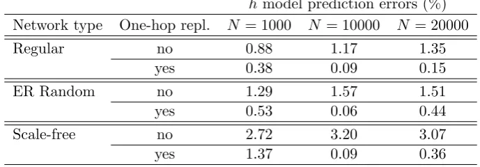
3.4.4 Dependency on the network size

Finally, we analyze the dependency of the average search length on the size of the network.

Sim-ulation experiments for networks of N = 1000 and N = 20000 nodes have been added to the base

experiments for N = 10000 nodes presented so far. Figure 5 show the average search length

ob-tained for regular, ER and scale-free networks as a function of their size. The average degree of all

1e+02 1e+03 1e+04 1e+05

1000 10000

average search length, log(hops)

All networks avg(k) = 10

Without one-hop replication

regular

1000 10000

network size, log(N) ER

1000 10000

RW (sim) (mod) SAW (sim) (mod)

scale-free

(a) Without one-hop replication.

1e+02 1e+03 1e+04

1000 10000

average search length, log(hops)

All networks avg(k) = 10

With one-hop replication

regular

1000 10000

network size, log(N) ER

1000 10000

RW (sim) (mod) SAW (sim) (mod)

scale-free

(b) With one-hop replication.

Figure 5: Average search length (h) as a function of network size.

hmodel prediction errors (%)

Network type One-hop repl. N = 1000 N = 10000 N = 20000

Regular no 0.88 1.17 1.35

yes 0.38 0.09 0.15

ER Random no 1.29 1.57 1.51

yes 0.53 0.06 0.44

Scale-free no 2.72 3.20 3.07

yes 1.37 0.09 0.36

Table 3: Relative errors of average search lengths predicted by the model with respect to simulation

results, for networks with k= 10.

It is observed that the average search length is linear in the network size. As for the previous

experiments, model predictions are in good agreement with simulation results. The magnitude of

deviations depends on the network type, on the presence of the one-hop replication feature and on

the network size. Table 3 presents these deviations relative to average search lengths registered in

simulations.

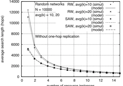
3.5 Several Instances of the Resource

We now look at the dependency of the average search length on the number of instances of the

resource sought present in the network (R). Figures 6(a) to 6(c) show this dependency for the three

types of networks, without one-hop replication, and for average degrees k = 10,20. Separately, to

networks with one-hop replication.

We observe that the reduction in h is large for the first additional resource instances,

asymp-totically tending to 0 as R grows towards the network size. (In particular, we have checked that

for SAW in networks without one-hop replication, this dependency is h_≈N/(R+ 1).) In networks

without one-hop replication, the difference in the average search length achieved by SAW and RW

quickly diminishes with the number of resource instances. A similar behavior can be observed in

networks with one-hop replication and with average degrees 10 and 20.

In these experiments, SAW searches outperform RW searches in networks without one-hop

replication regardless of their average degree. This is not true for networks with one-hop replication,

where an increase ink has a large impact on the rate at which the network is covered. This results

in a better performance of RW in networks with k= 20 than that of SAW in networks withk= 10.

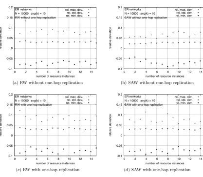
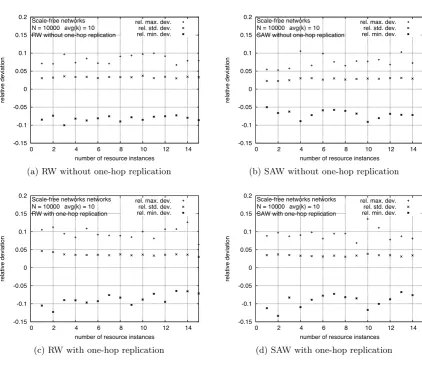
3.6 Variations of Network Averages

As stated in Section 2, our model of the SAW is a mean-field analysis that produces a estimation of

the average search length in networks with a given size and degree distribution. Of course, individual

walks on a given network can yield large deviations from the predicted average value. To ensure the

usefulness of the model when applied to an individual network (with the given degree distribution), the question that arises is now whether the choice of that particular topology can produce significant

deviations. To answer this question, Figure 7 (for ER random networks) and Figure 8 (for scale-free

networks) show deviations of network averages with respect to the value averaged over all networks

(the average search length,h). In particular, graphs show the standard deviation and the deviations

of the maximum and minimum values of network averages with respect to h. All deviations are

given relative toh. Recall from the description of the simulations (Section 3) thatnetwork averages

are values averaged over the 103 _{walks performed in each of the 10}2 _{individual networks. From}

these results it can be stated that the average search length predicted by the model for a given size

0 2000 4000 6000 8000 10000 12000

0 2 4 6 8 10 12 14

average search length (hops)

number of resource instances RW, avg(k)=10 (simul)

(model) RW, avg(k)=20 (simul) (model) SAW, avg(k)=10 (simul) (model) SAW, avg(k)=20 (simul) (model) Regular networks

N = 10000

avg(k) = 10, 20

Without one-hop replication

(a) Regular networks without one-hop replication

0 2000 4000 6000 8000 10000 12000 14000

0 2 4 6 8 10 12 14

average search length (hops)

number of resource instances RW, avg(k)=10 (simul)

(model) RW, avg(k)=20 (simul) (model) SAW, avg(k)=10 (simul) (model) SAW, avg(k)=20 (simul) (model) Random networks

N = 10000 avg(k) = 10, 20

Without one-hop replication

(b) ER random networks without one-hop replication

0 5000 10000 15000 20000

0 2 4 6 8 10 12 14

average search length (hops)

number of resource instances RW, avg(k)=20 (simul)

(model) RW, avg(k)=10 (simul) (model) SAW, avg(k)=20 (simul) (model) SAW, avg(k)=10 (simul) (model) Scale-free networks

N = 10000

avg(k) = 10, 20

Without one-hop replication

(c) Scale-free networks without one-hop replication

0 200 400 600 800 1000 1200 1400

0 2 4 6 8 10 12 14

average search length (hops)

number of resource instances RW, avg(k)=10 (simul)

(model) SAW, avg(k)=10 (simul) (model) RW, avg(k)=20 (simul) (model) SAW, avg(k)=20 (simul) (model) Regular networks

N = 10000 avg(k) = 10, 20

With one-hop replication

(d) Regular networks with one-hop replication

0 200 400 600 800 1000 1200 1400

0 2 4 6 8 10 12 14

average search length (hops)

number of resource instances RW, avg(k)=10 (simul)

(model) SAW, avg(k)=10 (simul) (model) RW, avg(k)=20 (simul) (model) SAW, avg(k)=20 (simul) (model) Random networks

N = 10000 avg(k) = 10, 20

With one-hop replication

(e) ER random networks with one-hop replication

0 200 400 600 800 1000 1200

0 2 4 6 8 10 12 14

average search length (hops)

number of resource instances RW, avg(k)=10 (simul)

(model) SAW, avg(k)=10 (simul) (model) RW, avg(k)=20 (simul) (model) SAW, avg(k)=20 (simul) (model) Scale-free networks

N = 10000

avg(k) = 10, 20

With one-hop replication

(f) Scale-free networks with one-hop replication

-0.1 -0.05 0 0.05 0.1 0.15 0.2

0 2 4 6 8 10 12 14

relative deviation

number of resource instances rel. max. dev.

rel. std. dev. rel. min. dev. ER networks

N = 10000 avg(k) = 10 RW without one-hop replication

(a) RW without one-hop replication

-0.1 -0.05 0 0.05 0.1 0.15 0.2

0 2 4 6 8 10 12 14

relative deviation

number of resource instances rel. max. dev.

rel. std. dev. rel. min. dev. ER networks

N = 10000 avg(k) = 10 SAW without one-hop replication

(b) SAW without one-hop replication

-0.1 -0.05 0 0.05 0.1 0.15 0.2

0 2 4 6 8 10 12 14

relative deviation

number of resource instances rel. max. dev.

rel. std. dev. rel. min. dev. ER networks

N = 10000 avg(k) = 10 RW with one-hop replication

(c) RW with one-hop replication

-0.1 -0.05 0 0.05 0.1 0.15 0.2

0 2 4 6 8 10 12 14

relative deviation

number of resource instances rel. max. dev.

rel. std. dev. rel. min. dev. ER networks

N = 10000 avg(k) = 10 SAW with one-hop replication

(d) SAW with one-hop replication

Figure 7: Relative deviations of network averages for search lengths in ER random networks with

-0.15 -0.1 -0.05 0 0.05 0.1 0.15 0.2

0 2 4 6 8 10 12 14

relative deviation

number of resource instances rel. max. dev.

rel. std. dev. rel. min. dev. Scale-free networks

N = 10000 avg(k) = 10 RW without one-hop replication

(a) RW without one-hop replication

-0.15 -0.1 -0.05 0 0.05 0.1 0.15 0.2

0 2 4 6 8 10 12 14

relative deviation

number of resource instances rel. max. dev.

rel. std. dev. rel. min. dev. Scale-free networks

N = 10000 avg(k) = 10 SAW without one-hop replication

(b) SAW without one-hop replication

-0.15 -0.1 -0.05 0 0.05 0.1 0.15 0.2

0 2 4 6 8 10 12 14

relative deviation

number of resource instances rel. max. dev.

rel. std. dev. rel. min. dev. Scale-free networks networks

N = 10000 avg(k) = 10 RW with one-hop replication

(c) RW with one-hop replication

-0.15 -0.1 -0.05 0 0.05 0.1 0.15 0.2

0 2 4 6 8 10 12 14

relative deviation

number of resource instances rel. max. dev.

rel. std. dev. rel. min. dev. Scale-free networks networks

N = 10000 avg(k) = 10 SAW with one-hop replication

(d) SAW with one-hop replication

Figure 8: Relative deviations of network averages for search lengths in scale-free networks with

4

Conclusions

We have proposed a mean-field model to estimate the average search length in randomly built

networks with a given size and degree distribution. The model considers the possible use of one-hop

replication and the existence of multiple resource instances. We have empirically evaluated the

model by generating networks of three types (regular, ER random and scale-free) and simulating

searches in them. We have found that the estimates are very accurate. When using SAW in networks with one-hop replication, the average search length decreases with the increase in average degree

for the three types of networks. In networks without one-hop replication, however, the impact of

average degree on the average search length is small, with slight decrements for ER random and

regular networks and slight increments for scale-free networks. Regarding the behavior with respect

to multiplicity of resource instances, the average search length is roughly inversely proportional to

the number of instances.

We have also simulated RW, with and without one-hop replication and with multiple resource

instances. The conclusion is that SAW has a much smaller average search length when one-hop replication is not available, especially in scale-free networks, where the reduction increases as the

average degree of the network grows. In networks with one-hop replication, reductions of average

search length are only significant for low average degrees, decreasing as the average degree grows.

The behavior with respect to the number of resource instances is similar to that of SAW.

An interesting future line to continue this work is to evaluate the search performance of variations

of the SAW, using different probability distributions for choosing the neighbor to visit next, e.g.,

based on combinations of its degree and of the number of times it has previously been visited or

covered.

5

References

References

[1] L.A. Adamic and B.A. Huberman, Zipf’s law and the internet, Glottometrics 3 (2002), 143–150.

[2] L.A. Adamic, R.M. Lukose, A.R. Puniyani, and B.A. Huberman, Search in power-law networks,

[3] M. Alanyali, V. Saligrama, and O. Savas, A random-walk model for distributed computation

in energy-limited networks, Proc First Workshop Informat Theory its Application, 2006, pp. .

[4] D.J. Aldous, Lower bounds for covering times for reversible markov chains and random walks,

J Theoret Probability 2 (1989), 91–100.

[5] D. Amit, G. Parisi, and L. Peliti, Asymptotic behavior of the ‘true’ self-avoiding walk, Physical

Review B 27 (1983), 1635–1645.

[6] A.L. Barab´asi and E. Bonabeau, Scale-free networks, Sci American 288 (May 2003), 60–69.

[7] G. Barnes and U. Feige, Short random walks on graphs, Proc Twenty-fifth Ann ACM Symp

Theory Comput (STOC 93), ACM Press, 1993, pp. 728–737.

[8] N. Bisnik and A. Abouzeid, Modeling and analysis of random walk search algorithms, Proc

Second Int Workshop Hot Topics in Peer-to-Peer Syst (Hot-P2P 2005), New York, New York,

United States, IEEE Computer Society, 2005, pp. 95–103.

[9] G. Brightwell and P. Winkler, Maximum hitting time for random walks on graphs, Random

Structures Algorithms 1 (1989), 263–276.

[10] J. Candia, P.E. Parris, and V.M. Kenkre, Transport properties of random walks on

scale-free/regular lattice hybrid networks, J Stat Phys 129 (2007), 323–333.

[11] Y. Chawathe, S. Ratnasamy, N. Lanham, and S. Shenker, Making gnutella-like p2p systems scalable, Proc 2003 Conference Appl, Technologies, Architectures, Protocols Comput Commun

(SIGCOMM), Karlsruhe, Germany, 2003, pp. 407–418.

[12] V. Cholvi, P.A. Felber, and E.W. Biersack, Efficient search in unstructured peer-to-peer

net-works, Proc Sixteenth Ann ACM Symp Parallelism in Algorithms Architectures, Barcelona, Spain, 2004, pp. 271–272.

[13] L. da Fontoura Costa and G. Travieso, Exploring complex networks through random walks,

Physical Review E 75 (2007).

[15] U. Feige, A tight lower bound on the cover time for random walks on graphs, Random Structures

Algorithms 6 (1995), 433–438.

[16] S. Fortunato and A. Flammini, Random walks on directed networks: The case of pagerank,

e-print physics (2006).

[17] C. Gkantsidis, M. Mihail, and A. Saberi, Random-walks in peer-to-peer networks: Algorithms

and evaluation, Performance Evaluation 63 (2006), 241–263.

[18] C.P. Herrero, Self-avoiding walks on scale-free networks, Physical Review E 71 (2005).

[19] B.D. Hughes, Random walks and random environments Vol. 1, Clarendon Press, Oxford, 1995.

[20] J.D. Kahn, N. Linial, N. Nisan, and M.E. Saks, On the cover time of random walks on graphs,

J Theoret Probability 2 (1989), 121–128.

[21] T. Kuczek and K. Crank, On a self-avoiding random walk, Indian J Stat 56 A (1994), 54–66.

[22] C. Law and K.Y. Siu, Distributed construction of random expander networks, Proc

Twenty-second Ann Joint Conference IEEE Comput Commun Societies (INFOCOM 2003), Vol. 3,

2003, pp. 2133–2143.

[23] S.H. Lee, P.J. Kim, and H. Jeong, Statistical properties of sampled networks, Physical Review

E 73 (2006).

[24] L. Lov´asz, “Random walks on graphs: A survey,” Combinatorics, Paul Erd˝os is eighty, Bolyai

Society Mathematical Studies, 2, Keszthely (Hungary), 1993, Vol. 2, pp. 1–46.

[25] Q. Lv, P. Cao, E. Cohen, K. Li, and S. Shenker, Search and replication in unstructured

peer-to-peer networks, Proc Sixteenth Int Conference Supercomputing, New York, New York, United

States, 2005, pp. 84–95.

[26] Q. Lv, S. Ratnasamy, and S. Shenker, Can heterogeneity make gnutella scalable?, Revised

papers from First Int Workshop Peer-to-Peer Syst, Cambridge, United States, 2002, pp. 94–

[27] I. Mabrouki, X. Lagrange, and G. Froc, Random walk based routing protocol for wireless sensor

networks, Proc Second Int Conference Performance Evaluation Methodologies Tooks

(Value-Tools ’07), ICST (Institute for Computer Sciences, Social-Informatics and Telecommunications

Engineering), 2007, pp. 1–10.

[28] N. Madras and G. Slade, The self-avoiding walk, Birkh¨auser, Boston, 1996.

[29] G.S. Manku, M. Naor, and U. Wieder, Know thy neighbor’s neighbor: The power of lookahead

in randomized p2p networks, Proc 36th Ann ACM Symp Theory Comput (STOC 2004), ACM

Press, 2004, pp. 54–63.

[30] R. Motwani and P. Raghavan,Markov chains and random walkschapter 6, pp. 127–160,

Cam-bridge University Press 1995.

[31] M.E.J. Newman, A.L. Barab´asi, and D.J. Watts, The structure and dynamics of networks, Princeton University Press, 2006.

[32] M.E.J. Newman, S.H. Strogatz, and D.J. Watts, Random graphs with arbitrary degree

distri-butions and their applications, Physical Review E 64 (2001).

[33] S.A. Pandit and R.E. Amritkar, Random spread on the family of small-world networks, Physical

Review E 63 (2001).

[34] M. Ripeanu, Peer-to-peer architecture case study: Gnutella network, Proc First Int Conference

Peer-to-Peer Comput, 2001, pp. 99–100.

[35] L. Rodero-Merino, A. Fern´andez Anta, L. L´opez, and V. Cholvi, Performance of random walks

in one-hop replication networks, Comput Networks 54 (2010), 781–796.

[36] N. Sadagopan, B. Krishnamachari, and A. Helmy, Active query forwarding in sensor networks, Ad hoc Networks 3 (2005), 91–113.

[37] N. Sarshar and V. Roychowdhury, Scale-free and stable structures in complexad-hocnetworks,

[38] G. Slade, The self-avoiding walk: A brief survey, Revised May 28, 2010. To appear in Surveys in

Stochastic Processes, Proceedings of the 33rd SPA Conference in Berlin, 2009, to be published

in the EMS Series of Congress Reports, eds. J. Blath, P. Imkeller, S. Roelly.

[39] G. Slade, The diffusion of self-avoiding random walk in high dimensions, Commun in Math

Phys 110 (1987), 661–683.

[40] B. Tadi´c, Adaptive random walks on the class of web graphs, Eur Physical J B 23 (2001),

221–228.

[41] S.J. Yang, Exploring complex networks by walking on them, Physical Review E 71 (2005).

[42] D. Zuckerman, A technique for lower bounding the cover time, Proc Twenty-second Ann ACM