SEISMIC LOADING
by Emilie Murphy
A thesis
submitted in partial fulfillment of the requirements for the degree of Master of Science in Mechanical Engineering
Boise State University
BOISE STATE UNIVERSITY GRADUATE COLLEGE
DEFENSE COMMITTEE AND FINAL READING APPROVALS
of the thesis submitted by
Emilie Murphy
Thesis Title: Dynamic Modeling of a Suspended and Shock Isolated System in Seismic Loading
Date of Final Oral Examination: 3 May 2019
The following individuals read and discussed the thesis submitted by student Emilie Murphy, and they evaluated her presentation and response to questions during the final oral examination. They found that the student passed the final oral examination.
John F. Gardner, Ph.D. Chair, Supervisory Committee Donald Plumlee, Ph.D. Member, Supervisory Committee Zhangxian Deng, Ph.D. Member, Supervisory Committee Jared D. Jeffrey, M.S. Member, Supervisory Committee
iv DEDICATION
I would like to dedicate this effort to the people who have supported me most throughout my educational endeavors. These people are my parents, Dave and Debbie, sister, Katelyn, and my grandparents, Richard and Geri Eismann. Not only have they supported my education financially, but they have supported and encouraged every dream and aspiration I have ever had. Even as a little girl, I was told I could accomplish
v
ACKNOWLEDGEMENTS
First and foremost, I would like to acknowledge the support, time, and assistance of Dr. John Gardner. I had the pleasure of taking Kinematics from Dr. Gardner during the junior year of my undergraduate degree. Throughout the tasks he assigned, he would give optional extra tasks where he’d say, “If you liked this, you should try…”. I pursued some of these extra tasks and discovered how much I enjoyed blending my Mechanical
Engineering major and Computer Science minor. After a few months in his class, he asked if I had ever considered applying to the Mechanical Engineering department’s Accelerated Masters program. Not only had I never considered a Master’s degree, I had never heard of this accelerated program. It was because of his support and encouragement that I applied and was later accepted into the program. He also encouraged me to pursue a Masters of Science instead of a Masters of Engineering and didn’t even bat an eye when I proposed doing an industry project unlike anything else anyone was doing in the graduate program. These moments and many more have been such important points in my life. I couldn’t be more grateful and thankful for his support and guidance through it all.
vi
vii ABSTRACT
A dynamic model for a suspended and shock isolated system is derived and implemented in MATLAB’s Simulink software. The purpose of this implementation is to create a design tool which is modularized to be able to accommodate any configuration of a similar system in any kind of loading. The design tool is used to compute the level of acceleration experienced at specific points in space within the system in the presence of seismic events, as typified by the dynamic displacement caused by the Sumatra,
viii
TABLE OF CONTENTS
DEDICATION ... iv
ACKNOWLEDGEMENTS ...v
ABSTRACT ... vii
LIST OF TABLES ... xi
LIST OF FIGURES ... xii
LIST OF ABBREVIATIONS ...xv
CHAPTER 1: INTRODUCTION ...1
Literature Review...2
Objective ...4
Description of System ...4
CHAPTER 2: TECHNICAL BACKGROUND ...9
Development of the Platform Model ...10
Rotation using the Euler Angle Method ...12
Equations of Motion using the Euler Angle Method ...14
Rotation using the Momentum Method ...15
Equations of Motion using the Momentum Method ...16
Development of the Shock Absorber Model ...17
Development of the Chain Model ...20
ix
CHAPTER 3: SIMULINK MODEL FORMULATION ...24
Model Initialization ...25
Platform Model Formulation ...27
Euler Angle Platform Model Formulation ...27
Derivation of State Platform Model Formulation ...30
Shock Absorber Model Formulation ...34
Chain Model Formulation ...36
World Model Formulation ...37
Sensor Formulation ...39
System Operation ...40
Model Verification ...40
Test Case 1: Equilibrium ...41
Test Case 2: Measured Movement in the Z Direction ...42
Test Case 3: Measured Movement in the X Direction ...44
Test Case 4: Measured Movement in the Y Direction ...45
Test Case 5: Asymmetric Configuration...46
CHAPTER 4: MODEL EXPERIMENTATION, TESTING, AND RESULTS...50
Earthquake Testing ...50
Parameter Sensitivity Study ...54
Chain Spring Constant Study ...55
Failure Case Study ...57
CHAPTER 5: APPLICATION OF MODEL ...60
x
Future Study ...61
CHAPTER 6: CONCLUSIONS ...62
REFERENCES ...64
xi
LIST OF TABLES
xii
LIST OF FIGURES
Figure 1. Deformation Modes of Tunnels During Seismic Events [2] ... 3
Figure 2. 3D Representation of System... 5
Figure 3. Labeled Platform Dimensions... 6
Figure 4. Labeled Shock Absorber Subsystem ... 7
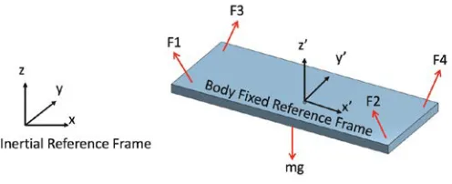
Figure 5. Platform Subsystem Coordinate Frames and FBD ... 11
Figure 6. Visualization of Roll-Pitch-Yaw Rotations [12]... 13
Figure 7. FBD of Shock Absorber Subsystem ... 17
Figure 8. Visualization of Spring Length Change ... 20
Figure 9. P and S Waves [16] ... 22
Figure 10. Model Flowchart ... 24
Figure 11. InitFcn Callback within Model Properties ... 27
Figure 12. Euler Angle Platform Model Overview ... 28
Figure 13. Initial Conditions for Position Integrator Blocks ... 30
Figure 14. Momentum Method Platform Model Overview ... 31
Figure 15. Momentum Method Platform Model Platform Angular Velocity Subsystem ... 32
Figure 16. Momentum Method Platform Model Rotation Matrix Calculator Subsystem ... 32
Figure 17. Momentum Method Platform Model Platform Linear Motion Subsystem ... 33
xiii
Figure 19. Shock Absorber Piston Location Integrator Block Parameters ... 35
Figure 20. Chain Subsystem Model Overview ... 36
Figure 21. World Displacement Subsystem Overview ... 39
Figure 22. Sensor Subsystem Overview... 40
Figure 23. Full System Overview... 40
Figure 24. Equilibrium Test Case Results ... 42
Figure 25. Measured Movement in the Z Direction Test Case Results ... 43
Figure 26. Measured Movement in Z Direction Chain Test Case Results ... 44
Figure 27. Measured Movement in the X Direction Test Case Results ... 45
Figure 28. Measured Movement in X Direction Euler Angle Test Case Results ... 45
Figure 29. Measured Movement in Y Direction Test Case Results ... 46
Figure 30. Measured Motion in Y Direction Euler Angle Comparison ... 46
Figure 31. Asymmetric Configuration Test Case CG Results ... 49
Figure 32. Asymmetric Configuration Test Case Chain Results ... 49
Figure 33. 2007 Sumatra Displacement Data ... 51
Figure 34. Sensor Locations within Platform System ... 51
Figure 35. Dynamic System Results of Sumatra Earthquake Displacement ... 52
Figure 36. Sensor Acceleration Results ... 53
Figure 37. Data Acceleration Results ... 53
Figure 38. System Performance for Varying Spring Constant and Damping Coefficient... 55
Figure 39. Chain Spring Constant Sensitivity Study Results ... 56
Figure 40. Chain Instability Comparison ... 57
xiv
xv
LIST OF ABBREVIATIONS
CG Center of Gravity
FBD Free Body Diagram
ft foot/feet
lb pound/pounds
s second
CHAPTER 1: INTRODUCTION
In engineering industry, there is more and more emphasis being placed on
computer aided design and system modeling as technology becomes readily available and easily accessible. This enables companies to obtain an accurate picture of what a final product might look like or how a system may act, saving a significant amount of time and money on failed physical prototypes. Computer aided design tools such as 3D modeling, finite element analysis, dynamic modeling, etc. can all be utilized to create anything you can imagine in a minimal amount of time.
The design tool that this work will be showcasing is that of dynamic modeling. Dynamic modeling is the process of utilizing mathematical equations to simulate how a system will respond under various physical constraints and loading scenarios. This analysis can also be used to analyze things such as how subsystems interact with each other or accelerations at specific locations within a system, etc. This information is critical, as it can be used to determine things such as the loading conditions under which a system will fail, which can in turn be used to redesign and implement protective measures against failure.
A system of this type was chosen due to its use by governments around the world as a means of protection and survival during extreme situations. Some of these situations include providing to a place to live safely in extreme physical situations, such as an earthquake or nuclear blast. Through the creation of a dynamic model to represent a system such as this underground bunker, questions such as survivability within the structure, Gs experienced by personnel during an event, and more can be answered.
By focusing on modularization of model subsystems and a straight forward user interface, a design tool can be created to allow for the analysis of any configuration of the system in any loading scenario, such as seismic loading. This work is also to act as an example of how modeling a system in this manner can be done quickly and play an important role in the physical simulation and subsequent analysis of both the components and personnel within the system.
Literature Review
Figure 1. Deformation Modes of Tunnels During Seismic Events [2]
Large scale shake table studies have been conducted [3–5] analyzing seismic activity acting on tunnels. These studies are largely focused on tunnel structural design, the soil composition, and their interaction with the underground structure. This can help in the reader’s understanding of underground structures in seismic events, but this work is more focused on what the system inside the structure experiences when systems such as shock absorbers are utilized to dampen an earthquake’s effects.
The system this work will be modeling is quite different from any other system found in literature review. One of the concepts that is most critical in the development of this dynamic model is the understanding of rigid body dynamics [10]. This
understanding, coupled with the use of two different methods [11] to represent the rotation of a rigid body through three-dimensional space will be used to create a dynamic model to represent the system. The mathematics behind these methods will be further described in the Technical Background section.
Objective
The objective of this work is to create a design tool which is modularized to be able to accommodate any configuration of a similar system in any kind of base excitation loading. The tool can then be used to analyze how the parameters within the system affect the motion and acceleration experienced at any location within the shock isolated
platform subsystem. Specifically, the desire of this analysis is to determine whether or not components and personnel within the platform subsystem will be able to survive a seismic event. Another desire of analysis is to determine how dependent the system is on its parameters to be able to create a priority list for maintenance to a current system or for development of a future system.
Description of System
configuration of this system can be seen in Fig. 2. The intent of a system configuration of this type is to reduce and absorb sudden and violent motion. This is done in part through the pendulum effect resulting from the suspension of the chains and also in part from the shock absorbers.
Figure 2. 3D Representation of System
Capsules which are used as the shell for underground bunkers are generally made of steel or steel rebar reinforced concrete. For our purposes, the makeup and general shape of the capsule are not considered. This is because the objective of this simulation is to analyze how the platform responds to motion of the anchor points of the chains and is not concerned with the capsule itself. The compression and ovaling described in the Literature Review section previously are not damage modes which are attempting to be mitigated with the shock absorber subsystem. Therefore, any motion experienced by the earth surrounding the capsule will be assumed to be the same motion experienced by the capsule.
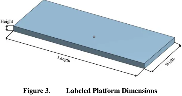
be rigid. The term “platform” will herein represent the platform and everything attached to it. With this assumption, the platform will be analyzed as a single rigid body. The dimensions of the platform are given hypothetical values of 25 ft long x 10 ft wide x 1 ft high. It is also given a hypothetical total weight of 4,000 lbs. Fig. 3 represents a platform with labeled dimensions.
Figure 3. Labeled Platform Dimensions
Rigidly attached to the top of the platform are four shock absorbers located in the four corners of the platform. The purpose of shock absorbers in a system such as this is to counteract and damp any force acting perpendicular to the platform through the shock. The shock absorbers are considered a separate subsystem from the platform because they are altering and modifying all force being transmitted through the chains to the platform.
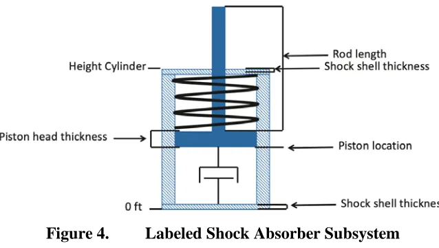
Shock absorbers vary widely in complexity and make up. A simple shock absorber was modeled for this hypothetical system. It is made up of a piston, oriented with the piston rod upward, a compression spring between the top of the inner cylinder volume and the top of the piston head, and a damping fluid between the bottom of the piston head and bottom of the inner cylinder volume. The configuration of this simple shock absorber can be viewed in Fig. 4. The shock absorber cylinder is given a
shell thickness of 1 inch (1 12
th foot). The shock absorber piston is given a head thickness
of 3 inches (1 4
th foot) and a rod length of 6.75 ft and 2 inches (1 6
th foot) in diameter. The
shock absorber is given a spring constant of 700 lb
ft and a damping coefficient of 150 lb∙s
ft . Every component within the shock absorber cylinder is assumed to be made of steel.
Figure 4. Labeled Shock Absorber Subsystem
Four chains are individually attached on one end to the top of each shock absorber piston rod and directly above each shock absorber to the inside of the capsule on the other end. These chains are assumed to be steel chain link. These four chains suspend the platform and shock absorber subsystems from the world around them. The chains also have the effect of making these subsystems act as a pendulum. Each chain is given a value for its unstretched length of 5 ft.
CHAPTER 2: TECHNICAL BACKGROUND
The study of dynamics is the study of how particles, bodies, and systems of bodies move and react when forces act upon them. It follows that a dynamic model is a computational design tool used to simulate how a particle, body, or system of bodies will move and react given the forces acting on the object over time. This is accomplished by deriving mathematical equations that represent how an object will act when excited. These mathematical equations are referred to as the model’s equations of motion. The excitation of the model over time is referred to as the model’s dynamic forcing function. The computational model uses initial conditions to create an initial state, then uses the forcing function to evaluate the equations of motion at each time step until the simulation time has expired.
The overall design intent behind the creation of a dynamic model is to best capture the nature of how a system acts while ensuring that all physical constraints imposed on the system are taken into account. There are many assumptions and
simplifications that can be made when creating and implementing a dynamic model that, when used appropriately, represents an otherwise very complex physical system without losing the system’s behavior. Simplifications can be regarding how a physical body may deflect, or even how a body moves, making the model easier to understand and
simplification is made, some accuracy can be lost within the model results. Therefore, assumptions must be made appropriately, when it is understood that the impact of said assumption will minimally impact the model’s results.
As a three-dimensional dynamic model for the chain, shock absorber, and platform system is being designed, how the model is going to be excited needs to be considered. This work is focusing on excitation through the displacement of seismic activity, recognized as base excitation [12]. The magnitude of the force due to
displacement will be calculated in the chain model and transmitted to the shock absorber model. Each shock absorber is rigidly attached to the platform and is therefore dependent on the orientation of the platform itself. The shock absorber model will take in the
transmitted chain forces and has the ability to counteract and damp any forces acting perpendicular to the platform orientation. It will then transmit these modified forces to the platform model. Those chain force components not perpendicular to the platform are transmitted directly to the platform, unmodified. The platform model will then take these forces transmitted at each shock absorber attach point and will calculate any resultant dynamic motion in the form of rotation and/or displacement of the platform itself. Any motion of the platform also results in the motion of each shock absorber and chain, as they are all connected in one system.
Development of the Platform Model
rigid body can undergo both translational and rotational motion, also known as general motion [13]. Any physical constraints on the amount of translation and rotation
experienced by the platform subsystem will be implemented through the platform’s interaction with the other subsystems within the system.
When working with rigid body dynamics in three-dimensional space, two different reference frames must be used. These two reference frames are the inertial reference frame and the body fixed reference frame. The inertial reference frame
represents the “world”, the origin of which can be located at any arbitrary point in space. A requirement of an inertial, or Newtonian, reference frame is that it is fixed or
translating with a constant velocity. The physical earth will be used to represent the inertial reference frame because the accelerations resulting from rotation about the sun are assumed to be small and therefore negligible [13]. The body fixed reference frame represents the rigid body, the origin of which is conventionally located at the body’s CG. Figure 5 further defines the two reference frames.
Figure 5. Platform Subsystem Coordinate Frames and FBD
force with a magnitude that is proportional to the force [13]. This can be expressed mathematically with the equation:
� 𝐹𝐹 =𝑚𝑚𝑚𝑚
where 𝐹𝐹 is representing the forces acting on the rigid body, 𝑚𝑚 represents the mass of the body, and 𝑚𝑚 is the acceleration of the body. When utilizing this law, it is a requirement that accelerations be computed with respect to the inertial reference frame. However, the forces acting on the body may be easier to calculate in the body fixed reference frame. For instance, the shock absorber subsystems can only counteract and damp forces that are perpendicular to the surface of the platform, or acting in the 𝑧𝑧′ axis of the body fixed reference frame as shown in Fig. 5. It is a much simpler process to calculate these forces in the body fixed frame and transform them to the inertial frame. This can be done through the use of the rotation transformation matrix.
The rotation transformation matrix is a construct of linear algebra which creates a mapping to move between the inertial and body fixed reference frames. In
three-dimensional space, this is represented by a 3-by-3 orthogonal square matrix. This matrix can be computed using a number of methods. The two methods utilized in this work are the Euler angle method and the momentum method.
Rotation using the Euler Angle Method
Figure 6. Visualization of Roll-Pitch-Yaw Rotations [12]
Using these angles, individual rotation matrices can be constructed to describe the rotation about each axis and then multiplied to represent the total rotation transformation matrix of the system. As derived by Ardakani and Bridges [12], these matrices are as follows:
𝑅𝑅𝜙𝜙 = �
1 0 0
0 cos𝜙𝜙 −sin𝜙𝜙
0 sin𝜙𝜙 cos𝜙𝜙 �
𝑅𝑅𝜃𝜃 = �
cos𝜃𝜃 0 sin𝜃𝜃
0 1 0
−sin𝜃𝜃 0 cos𝜃𝜃�
𝑅𝑅𝜓𝜓 = �
cos𝜓𝜓 −sin𝜓𝜓 0
sin𝜓𝜓 cos𝜓𝜓 0
0 0 1�
The total rotation transformation matrix is then represented as:
𝑄𝑄= 𝑅𝑅𝜓𝜓𝑅𝑅𝜃𝜃𝑅𝑅𝜙𝜙
𝑄𝑄 = �coscos𝜃𝜃𝜃𝜃cossin𝜓𝜓𝜓𝜓 sinsin𝜙𝜙𝜙𝜙sinsin𝜃𝜃𝜃𝜃sincos𝜓𝜓𝜓𝜓 −+ coscos𝜙𝜙𝜙𝜙cossin𝜓𝜓𝜓𝜓 coscos𝜙𝜙𝜙𝜙sinsin𝜃𝜃𝜃𝜃sincos𝜓𝜓 −𝜓𝜓+ sinsin𝜙𝜙𝜙𝜙cossin𝜓𝜓𝜓𝜓 −sin𝜃𝜃 sin𝜙𝜙cos𝜃𝜃 cos𝜙𝜙cos𝜃𝜃 �
Any vector can then be transformed from the body fixed frame to the inertial frame using the equation:
where 𝑒𝑒𝑏𝑏 is the vector in the body fixed frame and 𝑒𝑒𝑖𝑖 is the vector in the inertial frame. Transformation from the inertial to the body fixed frame can also be accomplished as follows:
𝑒𝑒𝑏𝑏 =𝑄𝑄𝑇𝑇𝑒𝑒𝑖𝑖
Equations of Motion using the Euler Angle Method
The first step in determining how the platform moves dynamically in response to the forces acting on it is to calculate the total moment acting on the platform in the body fixed frame. It is an assumption that all the force vectors transmitted to the platform are already in the body fixed frame. Therefore, the total moment can be easily calculated in the body fixed frame as:
𝑀𝑀= � 𝑟𝑟×𝐹𝐹𝐵𝐵
where 𝑟𝑟 is the position vector from the platform’s CG to the specific point where a shock absorber attaches to the platform and 𝐹𝐹 is the corresponding force transmitted by the shock absorber at that location. Due to the assumption that each component of the
platform subsystem is rigidly attached to the steel platform, it follows that the CG and the moment of inertia of the platform remain constant and unchanging in the body fixed frame. The angular acceleration, 𝛼𝛼𝐵𝐵, can then be solved for in the body fixed frame using Newton’s Second Law for Rotation:
𝛼𝛼𝐵𝐵= 𝐼𝐼𝑐𝑐−1(𝑀𝑀 − 𝜔𝜔𝐵𝐵×𝐻𝐻)
where 𝐼𝐼𝑐𝑐 is the inertia tensor, 𝜔𝜔𝐵𝐵 is the angular acceleration in the body fixed frame and
𝐻𝐻 is the angular momentum, which can be calculated as:
This angular acceleration can then be transformed into the inertial frame using the previously defined relation:
𝛼𝛼𝑖𝑖 =𝑄𝑄𝛼𝛼𝐵𝐵
From here, the angular acceleration in the inertial frame, 𝛼𝛼𝑖𝑖, can be integrated twice to obtain the Euler angles, 𝜙𝜙,𝜃𝜃, and 𝜓𝜓. Once the Euler angles are known, the original forces in the body fixed frame can be transformed into the inertial frame using the relation:
𝐹𝐹𝑖𝑖 =𝑄𝑄𝐹𝐹𝐵𝐵
With all necessary quantities now in the inertial frame, Newton’s Second Law can be used to calculate the acceleration, 𝑚𝑚, of the platform:
𝑚𝑚= 𝑚𝑚 1
𝑝𝑝𝑝𝑝𝑝𝑝𝑝𝑝𝑝𝑝𝑝𝑝𝑝𝑝𝑝𝑝� 𝐹𝐹𝑖𝑖
This acceleration can then be integrated twice to obtain the displacement of the platform’s CG in the inertial reference frame.
Rotation using the Momentum Method
Alternatively, a vector can be constructed in which all possible information necessary to represent a system is contained. This is referred to as the state vector. In this method, Baraff defines [10] the state vector, 𝑌𝑌(𝑡𝑡), and its derivative, 𝑑𝑑
𝑑𝑑𝑝𝑝𝑌𝑌(𝑡𝑡), for a rigid body to be:
𝑑𝑑 𝑑𝑑𝑡𝑡 𝑌𝑌(𝑡𝑡) = ⎝ ⎛ 𝑣𝑣(𝑡𝑡) 𝑅𝑅̇(𝑡𝑡) 𝐹𝐹(𝑡𝑡) 𝜏𝜏(𝑡𝑡)⎠ ⎞
where 𝑥𝑥(𝑡𝑡) is position, 𝑅𝑅(𝑡𝑡) is the rotation transformation matrix, 𝑃𝑃(𝑡𝑡) is the linear momentum, 𝐿𝐿(𝑡𝑡) is the angular momentum, 𝑣𝑣(𝑡𝑡) is the velocity, 𝐹𝐹(𝑡𝑡) is the force acting on the body, and 𝜏𝜏(𝑡𝑡) is the torque acting on the body. 𝑅𝑅̇(𝑡𝑡) is representing how the rotation matrix changes with time and can be calculated by using the equation:
𝑅𝑅̇(𝑡𝑡) =𝜔𝜔(𝑡𝑡)∗𝑅𝑅(𝑡𝑡)
where 𝜔𝜔(𝑡𝑡)∗ is a special angular velocity matrix defined as:
𝜔𝜔(𝑡𝑡)∗ =� 𝜔𝜔0 −𝜔𝜔𝑧𝑧 𝜔𝜔𝑦𝑦 𝑧𝑧 0 −𝜔𝜔𝑥𝑥
−𝜔𝜔𝑦𝑦 𝜔𝜔𝑥𝑥 0
�
Equations of Motion using the Momentum Method
By utilizing this method, calculations will be done almost exclusively in the inertial reference frame. Knowing the force experienced by the platform, linear
momentum can be directly solved for by integrating this force input. The velocity of the CG of the platform can then be calculated using the equation:
𝑣𝑣(𝑡𝑡) = 𝑚𝑚 𝑃𝑃(𝑡𝑡) 𝑝𝑝𝑝𝑝𝑝𝑝𝑝𝑝𝑝𝑝𝑝𝑝𝑝𝑝𝑝𝑝
where 𝑚𝑚𝑝𝑝𝑝𝑝𝑝𝑝𝑝𝑝𝑝𝑝𝑝𝑝𝑝𝑝𝑝𝑝 is the mass of the platform. This velocity can then be integrated to directly solve for the position of the CG of the platform.
𝜔𝜔(𝑡𝑡) =𝐼𝐼(𝑡𝑡)−1𝐿𝐿(𝑡𝑡)
where 𝐼𝐼(𝑡𝑡) is the platform’s inertia tensor in the inertial frame. As discussed previously, the platform’s inertia tensor is constant and easily computed in the body fixed frame. This inertia tensor can then be converted to the inertial frame using the relation:
𝐼𝐼(𝑡𝑡)𝑖𝑖𝑖𝑖𝑖𝑖𝑝𝑝𝑝𝑝𝑖𝑖𝑝𝑝𝑝𝑝 = 𝑅𝑅(𝑡𝑡)𝐼𝐼(𝑡𝑡)𝑏𝑏𝑝𝑝𝑑𝑑𝑦𝑦𝑝𝑝𝑖𝑖𝑥𝑥𝑖𝑖𝑑𝑑𝑅𝑅(𝑡𝑡)𝑇𝑇
Once these values are obtained, 𝜔𝜔(𝑡𝑡)∗ and 𝑅𝑅̇(𝑡𝑡) can be calculated and the new 𝑅𝑅(𝑡𝑡) obtained through the integration of 𝑅𝑅̇(𝑡𝑡).
Development of the Shock Absorber Model
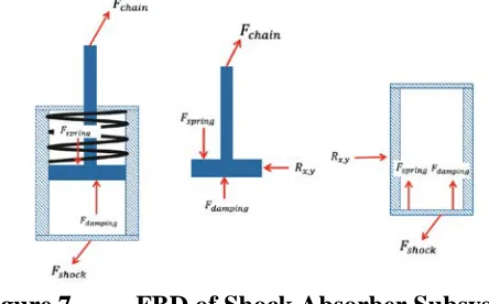
The goal of the shock absorber dynamic model is to determine how force input from the chains may be modified and then transmitted to the platform. To develop the equations of motion to represent this model, analysis must be done to determine how forces are being transmitted through the shock. This can be done in three steps: force analysis of the piston within the shock absorber, analysis of how these forces are transmitted to the shock absorber cylinder, followed by how the forces are transmitted from the cylinder to the platform. A free body diagram (FBD) of the forces acting on the shock absorber subsystem as a whole as well as on the piston and cylinder can be viewed in Fig. 7. These are two dimensional pictures to represent the three dimensional system.
An important first step in this process is to transform the input chain force acting at the top of the shock absorber piston from the inertial frame to the body fixed frame. This is due to the dependence of the shock absorbers on the orientation of the platform, represented by the body fixed frame. Forces can then be broken down into their 𝑥𝑥′,𝑦𝑦′, and 𝑧𝑧′ components for more straight forward analysis.
In the 𝑥𝑥′ and 𝑦𝑦′ directions, there is no acceleration of the shock absorber relative to the platform itself. Therefore, the two governing equations utilizing Newton’s Second Law in these directions become:
� 𝐹𝐹𝑥𝑥 = 0
� 𝐹𝐹𝑦𝑦 = 0
In both the 𝑥𝑥′ and 𝑦𝑦′ cases, the only forces acting on the system are the 𝑥𝑥′ and 𝑦𝑦′ component of the chain force and the resultant reaction forces from the shock absorber. From the chain to the shock absorber piston, the 𝑥𝑥′ and 𝑦𝑦′ component of the chain force would act equal in magnitude and opposite in direction. When the forces are transmitted from the piston to the shock absorber cylinder and then again from the cylinder to the platform, they act equal in magnitude and opposite in direction. This results in the following equations of motion in the 𝑥𝑥′ and 𝑦𝑦′ directions:
𝐹𝐹𝑠𝑠ℎ𝑝𝑝𝑐𝑐𝑜𝑜,𝑥𝑥 = 𝐹𝐹𝑐𝑐ℎ𝑝𝑝𝑖𝑖𝑖𝑖,𝑥𝑥′
𝐹𝐹𝑠𝑠ℎ𝑝𝑝𝑐𝑐𝑜𝑜,𝑦𝑦 = 𝐹𝐹𝑐𝑐ℎ𝑝𝑝𝑖𝑖𝑖𝑖,𝑦𝑦′
When analyzing the shock absorber piston in the 𝑧𝑧′ direction, there is an
the spring force and the damping force. The spring and damping forces will always be opposing the motion of the piston within the cylinder. Any force resulting from gravity acting on the piston is neglected, due to the assumption that the mass of the piston is significantly smaller than that of the platform. This results in the following equation of motion for the piston:
𝐹𝐹𝑐𝑐ℎ𝑝𝑝𝑖𝑖𝑖𝑖,𝑧𝑧′ − 𝐹𝐹𝑠𝑠𝑝𝑝𝑝𝑝𝑖𝑖𝑖𝑖𝑠𝑠− 𝐹𝐹𝑑𝑑𝑝𝑝𝑝𝑝𝑝𝑝𝑖𝑖𝑖𝑖𝑠𝑠 =𝑚𝑚𝑝𝑝𝑖𝑖𝑠𝑠𝑝𝑝𝑝𝑝𝑖𝑖𝑚𝑚𝑝𝑝𝑖𝑖𝑠𝑠𝑝𝑝𝑝𝑝𝑖𝑖
where 𝑚𝑚𝑝𝑝𝑖𝑖𝑠𝑠𝑝𝑝𝑝𝑝𝑖𝑖 and 𝑚𝑚𝑝𝑝𝑖𝑖𝑠𝑠𝑝𝑝𝑝𝑝𝑖𝑖 are the mass and acceleration of the piston, respectively. The spring force can be calculated as:
𝐹𝐹𝑠𝑠𝑝𝑝𝑝𝑝𝑖𝑖𝑖𝑖𝑠𝑠 =𝑘𝑘Δ𝑙𝑙
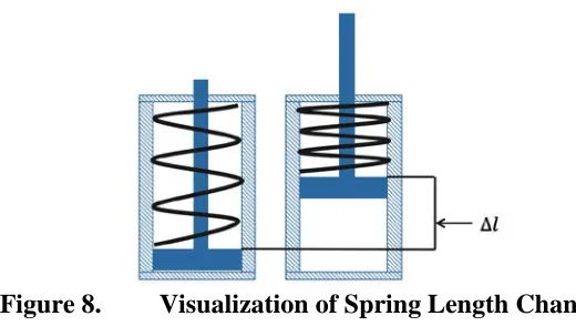
where 𝑘𝑘 is the spring constant and Δ𝑙𝑙 is the difference in length from the current location of the top of the piston head to location of the top of the piston head if it was resting on the bottom of the inner volume of the cylinder (i.e. the amount the spring has been compressed, assuming its free length is the equal to the maximum available length with the piston head resting on the bottom of the shock absorber cylinder). This can be best visualized through the use of Fig. 8. The damping force can be calculated as:
𝐹𝐹𝑑𝑑𝑝𝑝𝑝𝑝𝑝𝑝𝑖𝑖𝑖𝑖𝑠𝑠 = 𝑐𝑐𝑣𝑣𝑝𝑝𝑖𝑖𝑠𝑠𝑝𝑝𝑝𝑝𝑖𝑖
Figure 8. Visualization of Spring Length Change
When analyzing strictly the shock absorber cylinder the in the 𝑧𝑧′ direction, the forces acting are the spring force, the damping force, and the reaction force from the shock absorber. The reaction force from the shock absorber piston to the cylinder will act equal in magnitude and opposite in direction to the spring and damping forces. The direction of these forces will be reversed again when the forces are transferred from the shock absorber cylinder to the platform. The shock cylinder is also not accelerating relative to the platform. Therefore, the final equation of motion for the shock absorber subsystem is the following:
𝐹𝐹𝑠𝑠ℎ𝑝𝑝𝑐𝑐𝑜𝑜,𝑧𝑧 =𝐹𝐹𝑠𝑠𝑝𝑝𝑝𝑝𝑖𝑖𝑖𝑖𝑠𝑠+𝐹𝐹𝑑𝑑𝑝𝑝𝑝𝑝𝑝𝑝𝑖𝑖𝑖𝑖𝑠𝑠
Development of the Chain Model
This is a case where a full model to represent how the chains move dynamically can be very complex and computationally expensive [14]. In an effort to simplify the subsystem and obtain a quick and efficient simulation, assumptions and simplifications are made to this subsystem, making it the simplest subsystem in all.
move and/or rotate in reaction to the forces acting on it. Through the use of position vector algebra from the platform’s CG to the top of the shock absorber, the locations of the tops of the shock absorber pistons where the second end of the chains attach are also a known quantity. Therefore, the current length of each chain can be assessed using a simple position vector calculation from the top of the shock absorber piston to the location of the chain attach point on the inner surface of the capsule.
The next step is to quantify the forces generated due to any displacement of the capsule attach points. By analyzing how forces are transmitted through the chains, it can be observed that either 100% of force is transmitted when the chain is in tension or zero force is transmitted when the chain is slack. This is due to the chain not being a rigid body, such as a steel rod, and not being able to compress. Unfortunately, switches such as this where the force is either “on” or “off” can be very challenging to successfully model due to the discontinuities they cause. Instead of modeling the chain as a switch, the chain can be modeled as a very stiff spring, allowing for a slight compliance.
Utilizing the above simplifications, the model to represent the chain can be obtained. If the chain is in tension and being “stretched”, the force transmitted by the chain can be calculated as:
𝐹𝐹𝑐𝑐ℎ𝑝𝑝𝑖𝑖𝑖𝑖 =𝑘𝑘𝑐𝑐ℎ𝑝𝑝𝑖𝑖𝑖𝑖(𝑙𝑙𝑐𝑐𝑐𝑐𝑝𝑝𝑝𝑝𝑖𝑖𝑖𝑖𝑝𝑝− 𝑙𝑙0)
where 𝑘𝑘𝑐𝑐ℎ𝑝𝑝𝑖𝑖𝑖𝑖 is the spring constant of the chain, 𝑙𝑙𝑐𝑐𝑐𝑐𝑝𝑝𝑝𝑝𝑖𝑖𝑖𝑖𝑝𝑝 is the current length of the chain calculated using the chain position vector, and 𝑙𝑙0 is the unstretched length of the chain. If the chain is slack, then the force transmitted by the chain can be expressed as:
Development of the Seismic Forcing Function
Developing the seismic forcing function for this simulation is dependent on determining the displacement caused by a seismic event. The energy released during an earthquake is propagated through the crust of the earth in the form of two different waves, causing displacement. These are primary waves, “P waves”, taking the form of compression waves, and secondary waves, “S waves”, taking the form of transverse, or shear, waves [15]. This can be represented through the graphic in Fig. 9.
Figure 9. P and S Waves1 [16]
The momentum equation for a seismic wave can be represented as [16]:
𝑢𝑢̈ =𝛼𝛼2∇∇ ∙ 𝑢𝑢 − 𝛽𝛽2∇×∇×𝑢𝑢
where 𝑢𝑢 is the displacement, 𝑢𝑢̈ is the acceleration, ∇ is the gradient, 𝛼𝛼 is the P-wave velocity calculated as:
𝛼𝛼2 =𝜆𝜆+ 2𝜇𝜇
𝜌𝜌
and 𝛽𝛽 is the S-wave velocity calculated as:
𝛽𝛽2 =𝜇𝜇
𝜌𝜌
where 𝜆𝜆 and 𝜇𝜇 are Lamé coefficients and 𝜌𝜌 is the density. The calculations involved in these equations to model a seismic event in three dimensions can be very intensive.
Alternatively, displacement data gathered directly from seismographs can be utilized. This data can be searched for and downloaded from sources such as the U.S. Geological Survey (USGS). Three separate data files representing displacement in the east-west, north-south, and up-down directions can be manipulated and compiled together to create the total displacement experienced. These files also include necessary
CHAPTER 3: SIMULINK MODEL FORMULATION
MATLAB’s simulation software, Simulink [17], was chosen to be used for the formulation of a dynamic model to represent the system. There are two design goals behind the model to make it an effective and worthwhile design tool for the end user. The first goal is to focus on the modularization of each subsystem to allow for the subsystems to be arranged in any configuration. The second goal is to create an easy and straight forward user interface to allow for quick manipulation of the system parameters. This can be done through the use of initialization scripts, the details of which will be further discussed later. The formulation of each subsystem’s model in Simulink will be
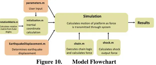
presented. This is then followed by an overview of system operation, describing how the model components work together. All code discussed in this section can be found in Appendix A. A flowchart of how the model and its supporting functions and scripts work together is shown in Fig. 10. Orange boxes are used in this figure to represent scripts that require input from the user.
Model Initialization
There are many parameters which make up the system, such as the length, width, and height of the platform, or the spring and damping coefficients of the shock absorber, etc. All of these parameters will be provided by the user and need to be in one easily accessible location. This is done by declaring all the system parameters in a script called “parameters.m”. Some of the parameters entered by the user include the location of the CG and the platform attach points, where the shock absorbers are attached. These
coordinates are entered in the “platform coordinate system”, with the origin in the bottom front left corner of the platform, instead of the convention with the origin located at the CG of the platform. This was a choice made by the model designer based on the
assumption that these coordinates and the moment of inertia could be easily obtained from a 3D CAD model of the subsystem. Using this method, components making up the configuration of the platform subsystem can be quickly modified within the 3D CAD model and the modified parameters could be swiftly obtained and updated for model simulation.
Any other parameters used by the model during simulation that are calculated from the user given parameters are located in an additional script called
“initialization.m”. System parameters calculated in this initialization script are values such as position vectors between the platform attach points and the platform’s CG in the body fixed frame. Also calculated in this script is the initial location of the platform CG in the inertial reference frame. This is done by defining a plane in three dimensional space using three of the chain attach points and calculating the normal vector to the plane,
𝑠𝑠 =�chain attach point 1 ychain attach point 1 x
chain attach point 1 z�,𝑡𝑡 =�
chain attach point 2 x chain attach point 2 y
chain attach point 2 z�,𝑢𝑢
=�chain attach point 3 xchain attach point 3 y
chain attach point 3 z�
𝑛𝑛 = (𝑡𝑡 − 𝑠𝑠) × (𝑢𝑢 − 𝑠𝑠)
Any initial rotations in the platform resulting from an asymmetric configuration of the system can then be calculated using the equations:
𝜙𝜙𝑝𝑝= sin�−𝑛𝑛𝑛𝑛 𝑦𝑦 𝑧𝑧 �
𝜃𝜃𝑝𝑝= sin�−𝑛𝑛𝑛𝑛 𝑥𝑥 𝑧𝑧 �
There is no configuration of the system that could cause an initial rotation about the z axis. From these rotations, the inertial CG can be calculated.
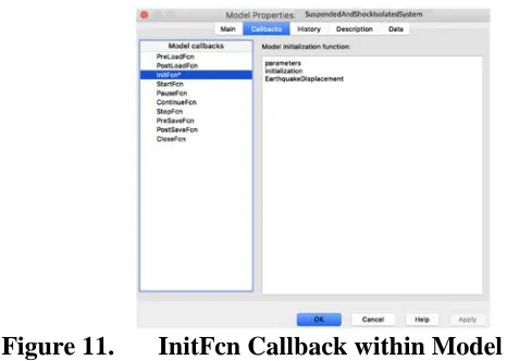
Figure 11. InitFcn Callback within Model Properties
The initialization script titles are placed within the “Model initialization function” box in the order in which they need to be run. The “EarthquakeDisplacement” script will be discussed in the World Model Formulation section later.
Platform Model Formulation
As discussed in the Development of the Platform Model section, there are two sets of equations of motion which can be used to represent the dynamic motion of the platform, resulting from the two rotation transformation matrix methods utilized in this work. There are therefore two different Simulink platform models that can be formulated. The input for each platform model will be the four force vectors in the body fixed
reference frame and the four 𝑧𝑧′ distances from the platform attachment point to the top of the shock absorber piston attach point from each of the four shock absorbers. The output of each model will be the location of each shock absorber piston attach point in the inertial reference frame.
Euler Angle Platform Model Formulation
acting on the body to determine the angular acceleration of the platform in the body fixed frame. This total moment acting on the body is calculated using the equation:
𝑀𝑀 =𝑟𝑟1 ×𝐹𝐹1+𝑟𝑟2×𝐹𝐹2+𝑟𝑟3×𝐹𝐹3+𝑟𝑟4×𝐹𝐹4
where 𝑟𝑟 is the position vector from the platform’s CG to the respective shock absorber piston attach points and 𝐹𝐹 is the force vector for the respective points in the body fixed frame. The angular acceleration in the body fixed frame can then be calculated using the previously described equation:
𝛼𝛼𝐵𝐵= 𝐼𝐼𝑐𝑐−1(𝑀𝑀 − 𝜔𝜔𝐵𝐵×𝐻𝐻)
where 𝜔𝜔𝐵𝐵 is the angular acceleration in the body fixed frame and 𝐻𝐻 is the angular
momentum of the platform. The model uses the initial condition that there is zero angular velocity to solve the first time step.
Figure 12. Euler Angle Platform Model Overview
The angular acceleration in the body fixed frame is then sent to the Euler Angle Calculator function to be transformed into the inertial frame. This is accomplished using the relation:
where 𝑅𝑅 is the rotation transformation matrix calculated using Euler angles. This function utilizes the initial condition that 𝜙𝜙,𝜃𝜃, and 𝜓𝜓 are zero to solve the first time step. The inertial angular acceleration values are then integrated twice to obtain the Euler angles. A function script named “rotationMatrix.m” is utilized in this function, in which the Euler angles are passed to the function, the total rotation transformation matrix is calculated, and then the rotation transformation matrix is returned. This function is used to reduce unnecessary code duplication.
The Euler angles can now be used to solve for the translational acceleration of the platform by transforming the inputted forces from the body fixed frame to the inertial frame. Translational acceleration can be solved for using the equation:
𝑚𝑚=𝑚𝑚 1
𝑝𝑝𝑝𝑝𝑝𝑝𝑝𝑝𝑝𝑝𝑝𝑝𝑝𝑝𝑝𝑝(𝐹𝐹1+𝐹𝐹2+𝐹𝐹3+𝐹𝐹4− 𝐹𝐹𝑤𝑤𝑖𝑖𝑖𝑖𝑠𝑠ℎ𝑝𝑝)
where 𝐹𝐹𝑤𝑤𝑖𝑖𝑖𝑖𝑠𝑠ℎ𝑝𝑝 can be calculated as the platform weight vector:
𝐹𝐹𝑤𝑤𝑖𝑖𝑖𝑖𝑠𝑠ℎ𝑝𝑝= � 0 0
𝑚𝑚𝑝𝑝𝑝𝑝𝑝𝑝𝑝𝑝𝑝𝑝𝑝𝑝𝑝𝑝𝑝𝑝𝑔𝑔
�
Figure 13. Initial Conditions for Position Integrator Blocks
Once the location of the platform CG is known in the inertial frame, the updated location of the shock absorber piston attach points can be calculated in the Platform World Coordinates function. This is done using simple vector algebra, adding the position vectors together with the CG of the platform. The platform attach points are calculated so they can be sent to the MATLAB base workspace in the form of timeseries data arrays. These arrays can then be used by post processing scripts, such as an
animation script to assist in the visualization of the system’s motion. The shock absorber piston locations and the platform’s Euler angles can then be outputted for use by the rest of the system.
Derivation of State Platform Model Formulation
An overview of the platform Simulink model utilizing the derivation of state method is shown in Fig. 14. The first step of this model is to calculate the total force and total moment acting on the platform in the inertial frame within the Total Force and Moment function. This can be done using the equations:
𝐹𝐹𝑝𝑝𝑝𝑝𝑝𝑝𝑝𝑝𝑝𝑝 =𝑅𝑅(𝐹𝐹1+𝐹𝐹2+𝐹𝐹3+𝐹𝐹4)− 𝐹𝐹𝑤𝑤𝑖𝑖𝑖𝑖𝑠𝑠ℎ𝑝𝑝
where 𝑟𝑟 is the position vector from the platform’s CG to the respective shock absorber piston attach points, 𝐹𝐹 is the force vector for the respective points in the body fixed frame, and 𝑅𝑅 is the total rotation transformation matrix.
Figure 14. Momentum Method Platform Model Overview
The total moment is then passed to the Platform Angular Velocity group, along with the total rotation transformation matrix, shown in Fig. 15. The total moment is integrated to obtain the angular momentum of the platform. The platform’s angular velocity can be calculated by rotating the platform’s inertia tensor into the inertial frame and using the equation:
𝜔𝜔(𝑡𝑡) =𝐼𝐼(𝑡𝑡)−1𝐿𝐿(𝑡𝑡)
Figure 15. Momentum Method Platform Model Platform Angular Velocity Subsystem
The angular velocity is then passed to the Rotation Matrix Calculator group, shown in Fig. 16, where 𝑅𝑅̇ can be calculated by using the equations:
𝜔𝜔(𝑡𝑡)∗ =� 𝜔𝜔0𝑧𝑧 −𝜔𝜔0𝑧𝑧 −𝜔𝜔𝜔𝜔𝑦𝑦𝑥𝑥
−𝜔𝜔𝑦𝑦 𝜔𝜔𝑥𝑥 0
�
𝑅𝑅̇(𝑡𝑡) =𝜔𝜔(𝑡𝑡)∗𝑅𝑅(𝑡𝑡)
Each component of 𝑅𝑅̇ can be integrated to obtain the total rotation transformation matrix,
𝑅𝑅. This updated rotation transformation matrix can then be outputted from the subsystem for use by the rest of the model.
Figure 16. Momentum Method Platform Model Rotation Matrix Calculator Subsystem
The translational velocity and position of the platform’s CG can be calculated within the Platform Linear Motion group, seen in Fig. 17. Here, the total force can be integrated and multiplied by 1
𝑝𝑝𝑝𝑝𝑝𝑝𝑝𝑝𝑝𝑝𝑝𝑝𝑝𝑝𝑝𝑝𝑝𝑝 to obtain the velocity of the CG. The velocity can
again done by using the initial location of the platform CG, calculated by “initialization.m”, as previously shown in Fig. 11.
Figure 17. Momentum Method Platform Model Platform Linear Motion
Subsystem
Knowing the location of the platform’s CG in the inertial frame, the location of the shock absorber piston attach points can be calculated within the Shock Position Calculator function. This is done using vector algebra, as described in the Euler angle platform model method.
For comparison of Euler angle results between the two platform models, the Euler angles can be calculated from the total rotation transformation matrix. Slabaugh’s method [18] was utilized in the Euler Angle Calculator function with the following equations:
𝜃𝜃= −sin−1(𝑅𝑅 3,1)
𝜙𝜙= tan−12�𝑅𝑅3,2 cos𝜃𝜃,
𝑅𝑅3,3
cos𝜃𝜃�
𝜓𝜓= tan−12�𝑅𝑅2,1 cos𝜃𝜃,
𝑅𝑅1,1
cos𝜃𝜃�
Shock Absorber Model Formulation
The goal of the shock absorber Simulink model is to modify the inputted force from the chain, based on the orientation of the shock absorber, and output the resultant force to the platform. An overview of a shock absorber model is shown in Fig. 18.
Figure 18. Shock Absorber Subsystem Model Overview
The first step of the Shock Force and Piston Acceleration Calculator function is to rotate the inputted chain force from the inertial frame to the body fixed frame. The
outputted resultant force in the body fixed frame and the piston acceleration can then be calculated within the function utilizing a function script “shock.m” using the following equations:
𝑚𝑚𝑝𝑝𝑖𝑖𝑠𝑠𝑝𝑝𝑝𝑝𝑖𝑖 =𝑚𝑚 1
𝑝𝑝𝑖𝑖𝑠𝑠𝑝𝑝𝑝𝑝𝑖𝑖�𝐹𝐹𝑐𝑐ℎ𝑝𝑝𝑖𝑖𝑖𝑖,𝑧𝑧′ − 𝐹𝐹𝑠𝑠𝑝𝑝𝑝𝑝𝑖𝑖𝑖𝑖𝑠𝑠− 𝐹𝐹𝑑𝑑𝑝𝑝𝑝𝑝𝑝𝑝𝑖𝑖𝑖𝑖𝑠𝑠�
𝐹𝐹𝑠𝑠ℎ𝑝𝑝𝑐𝑐𝑜𝑜= �
𝐹𝐹𝑐𝑐ℎ𝑝𝑝𝑖𝑖𝑖𝑖,𝑥𝑥′
𝐹𝐹𝑐𝑐ℎ𝑝𝑝𝑖𝑖𝑖𝑖,𝑦𝑦′
𝐹𝐹𝑠𝑠𝑝𝑝𝑝𝑝𝑖𝑖𝑖𝑖𝑠𝑠+𝐹𝐹𝑑𝑑𝑝𝑝𝑝𝑝𝑝𝑝𝑖𝑖𝑖𝑖𝑠𝑠
�
confines of the cylinder itself, initial conditions and integration restrictions are placed on the piston location integrator block as shown in Fig. 19. Setting these initial conditions to zero forces the system to find its equilibrium position, but does not impact the dynamic response of the system.
It is also assumed that when the spring is fully compressed, it takes up the distance of about two piston head thicknesses. It is important to note that although these restrictions will keep the location data in the correct ranges, the correct physics will not be captured if the piston is in an extreme enough situation where the piston head hits either the top or bottom of the inner shock volume (i.e. the acceleration will not reach zero and a resultant impact force is not calculated). To prevent this phenomenon from occurring, if the piston location is within the last foot of the cylinder, the spring constant is multiplied by 3 to represent the nonlinearity known as spring hardening. The piston location is then sent to the Z Distance Calculator function to determine the z distance from the bottom of the shock absorber to the top of the shock piston attach point.
Chain Model Formulation
The chain Simulink Model is a simple model whose overview can be seen in Fig. 20. The input to the model is the inertial location of the capsule attach point and the shock absorber piston attach point. These are passed to the Chain 1 function, where the “chain.m” function script is utilized to determine whether the chain is in tension or slack and what force is then outputted to the shock absorber. This transmitted force resulting from the chain being ‘stretched’ while in tension is calculated using the equation:
𝐹𝐹𝑐𝑐ℎ𝑝𝑝𝑖𝑖𝑖𝑖 =𝑘𝑘𝑐𝑐ℎ𝑝𝑝𝑖𝑖𝑖𝑖(𝑙𝑙𝑐𝑐𝑐𝑐𝑝𝑝𝑝𝑝𝑖𝑖𝑖𝑖𝑝𝑝− 𝑙𝑙0)
if the chain is in tension. The direction cosines of the position vector are then used to break down the chain force to its x, y, and z components. If the chain is slack, the chain force becomes:
𝐹𝐹𝑐𝑐ℎ𝑝𝑝𝑖𝑖𝑖𝑖 =� 0 0 0�
Figure 20. Chain Subsystem Model Overview
The spring constant for the chain was calculated from Young’s modulus of elasticity for steel. Using the relationship 𝜎𝜎= 𝐸𝐸𝐸𝐸, the spring constant can be calculated using the equation:
where Young’s modulus of carbon steel, 𝐸𝐸, is 30 Mpsi [19], the area is the cross sectional area of a chain link, 𝐴𝐴, can be calculated:
𝐴𝐴= 2(𝜋𝜋𝑟𝑟2)
with a chain radius of 0.25 inches, and a length, 𝐿𝐿, of 5 feet. The spring constant is calculated to be 2,401,920 lb
ft. This spring constant is much too stiff for the simulation and causes instabilities within the system. The value was reduced till a reasonable stability was achieved in the model and a spring constant of 20,000 lb
ft was chosen. Verification of this assumption will be discussed in the Parameter Sensitivity Study section.
World Model Formulation
The Simulink world model is where the forcing function of our simulation resides. The forcing function of this model is the displacement caused by an earthquake event. Earthquake data for this analysis was directly searched and downloaded from the Strong-Motion Virtual Data Center [20]. These files are downloaded as .smc files, which can be opened using any basic text editor. These files contain a lot of important
information, such as the title and magnitude of the earthquake, as well as the sample rate in which the data was collected [21]. Three displacement files express the three
dimensional earthquake displacement, where “HNN” in the file title is the North-South displacement, “HNE” is the East-West displacement, and “HNZ” is the up-down
displacement. The data from these three data files was scraped and concatenated into one .csv file with each row representing the x, y, and z displacement (i.e. East-West, North-South, and up-down) for each time step.
The data was acquired by Caltech Tectonics Observatory and processed by USGS National Strong Motion Project from sensors located on Sikuai Island, West Sumatra. Data was collected at a sample rate of 200 samples per second with 129 seconds of the event observed. This displacement data can be loaded into the model workspace through the use of “EarthquakeDisplacement.m” as an initialization script in the initialization function callback properties of the model, shown in Fig. 11. This script loads in the .csv file created from the earthquake displacement files, converts the file from centimeters to inches, and creates data arrays for the x, y, and z, displacement data with 4 seconds of delay, where no displacement is experienced. This delay is to allow the system model to settle and find its equilibrium. It also adds 50 seconds at the end of the simulation where the displacement is set to the last value of the earthquake displacement, to allow for the model to again settle.
An overview of the World Displacement subsystem is shown in Fig. 21. The displacement vectors can be loaded from the model workspace and passed to the Earthquake Displacement Data ReadIn function. This function selects the current displacement from the total displacement vectors and outputs them to the World Attachment Location Calculator function. The displacement is equally applied to all attachment locations at each timestep. This is because the velocities of P and S waves are on the order of 14,665 ft
s (4.47 km
s ) and 8,464 ft
s (2.58 km
s ) respectively [22]. With the capsule attach points about 8-23 ft apart, this displacement will be felt 1.5-2.7
Figure 21. World Displacement Subsystem Overview
Sensor Formulation
A major focus of this model is to be able to measure the accelerations experienced at any location within the platform subsystem. This can be accomplished by using a sensor subsystem. An overview of this subsystem is shown in Fig. 22. In this subsystem, the platform CG’s angular velocity and angular acceleration are passed to the Sensor Velocity and Acceleration Calculator function. Because the sensor is representing a location rigidly attached to the platform subsystem and the platform is rotating around its CG, the acceleration of a single point within this body can be calculated using the
equations [13]:
𝑣𝑣 =𝜔𝜔×𝑟𝑟
𝑚𝑚=𝛼𝛼×𝑟𝑟+𝜔𝜔× (𝜔𝜔×𝑟𝑟)
where 𝜔𝜔 is the angular velocity of the CG, 𝛼𝛼 is the angular acceleration of the CG, and 𝑟𝑟 is the position vector from the CG to the sensor location. The calculated acceleration is then sent to the Conversion to g’s function where it is converted from ft
Figure 22. Sensor Subsystem Overview
System Operation
Finally, all of the subsystem components can be connected together to form a full dynamic model. The full system overview is shown in Fig. 23. By utilizing the
modularized subsystems in this way, each system acts independently while adhering to the necessary physical constraints. Forces are transmitted down from the earthquake displacement through the chains, modified by the shock absorbers, to the platform. The platform then moves dynamically and the location of the system components are updated.
Figure 23. Full System Overview
Model Verification
that deal with platform rotation can be very challenging. To do this, results from using the Euler angle mentod platform model will be compared with results obtained from using the momentum method platform model to verify their accuracy.
Test Case 1: Equilibrium Set Up
Using the parameters described in the Description of System section of this work, the equilibrium state of the system can be verified. To test the equilibrium case, zero displacement will be sent to the World Attachment Location Calculator function within the World Displacement subsystem to allow for the system to find its equilibrium. This settling of the system is due to movement of the pistons within the shock absorber
cylinders as the springs are compressed until they balance the weight of the platform. The amount the platform will be displaced can be calculated as follows:
Δ𝑙𝑙 =𝐹𝐹𝑤𝑤𝑖𝑖𝑖𝑖𝑠𝑠ℎ𝑝𝑝
𝑘𝑘
where 𝑘𝑘 is the spring constant and 𝐹𝐹𝑤𝑤𝑖𝑖𝑖𝑖𝑠𝑠ℎ𝑝𝑝 is the weight of the platform. The spring constant can be calculated after analyzing that the 4 chains act in parallel and the 4 shock absorber springs act in parallel, while the chain and shock absorber springs act in series with each other. This k can be calculated as [12]:
𝑘𝑘𝑐𝑐ℎ𝑝𝑝𝑖𝑖𝑖𝑖,𝑝𝑝𝑝𝑝𝑝𝑝𝑝𝑝𝑝𝑝 = 4𝑘𝑘𝑐𝑐ℎ𝑝𝑝𝑖𝑖𝑖𝑖
𝑘𝑘𝑠𝑠ℎ𝑝𝑝𝑐𝑐𝑜𝑜,𝑝𝑝𝑝𝑝𝑝𝑝𝑝𝑝𝑝𝑝 = 4𝑘𝑘𝑠𝑠ℎ𝑝𝑝𝑐𝑐𝑜𝑜
𝑘𝑘= 𝑘𝑘𝑘𝑘𝑐𝑐ℎ𝑝𝑝𝑖𝑖𝑖𝑖,𝑝𝑝𝑝𝑝𝑝𝑝𝑝𝑝𝑝𝑝𝑘𝑘𝑠𝑠ℎ𝑝𝑝𝑐𝑐𝑜𝑜,𝑝𝑝𝑝𝑝𝑝𝑝𝑝𝑝𝑝𝑝 𝑐𝑐ℎ𝑝𝑝𝑖𝑖𝑖𝑖,𝑝𝑝𝑝𝑝𝑝𝑝𝑝𝑝𝑝𝑝+𝑘𝑘𝑠𝑠ℎ𝑝𝑝𝑐𝑐𝑜𝑜,𝑝𝑝𝑝𝑝𝑝𝑝𝑝𝑝𝑝𝑝
fall past its equilibrium point, experience a slight overshoot as it is pulled back upwards by the chains, and then settle to its equilibrium state.
Results
The expected results are corroborated by the simulation, as shown in Fig. 24. The platform’s CG begins at -12.583 ft in the z direction and after 4 seconds has reached an equilibrium state of -14.062 ft.
Figure 24. Equilibrium Test Case Results
Test Case 2: Measured Movement in the Z Direction Set Up
Results
The expected results are corroborated by the simulation, as shown in Fig. 25. The significant displacement at 4 seconds when the step function is applied is due to the very high spring constant of the chains. At 8 seconds, the system reaches its new equilibrium of -13.562 ft. The total forces in each chain are shown in Fig. 26. These results show that when the instantaneous displacement takes place, a large force is generated within the chains, resulting in the platform being sharply pulled upward. Once the chains have pulled the platform upward, the platform’s momentum continues upward, resulting in the chains being slack and their forces going to zero for a few milliseconds. During this short time, the platform experiences freefall where it is affected by gravity alone. Once the chains are again in tension, the system again settles to its new equilibrium position.
Figure 26. Measured Movement in Z Direction Chain Test Case Results
Test Case 3: Measured Movement in the X Direction Set Up
After letting the system reach equilibrium, a step function will apply a 6 inch displacement in the positive x direction. This is expected to result in the x coordinate for the platform’s CG to oscillate until reaching a new equilibrium from 11.5 to 12 ft. The x coordinate is expected to oscillate due to the platform rotations which develop from the sudden x movement. There are no mechanisms within the system to directly damp movement or forces in the x or y directions. However, the motion in the x direction is expected to be damped out over time and reach an equilibrium. This is because with each rotation about the y axis, a small component of the side loads applied to the system will act in the 𝑧𝑧′ direction of the body fixed frame, which will be damped by the shock absorbers.
Results
location of the CG’s x coordinate can be seen to oscillate, trending towards 12 ft after 30 seconds of simulation. The amplitude of these oscillations is also observed to be damped as the simulation time progresses. The Euler Angles can also be compared in Fig. 28 and although very small, rotation only about the y axis is observed.
Figure 27. Measured Movement in the X Direction Test Case Results
Figure 28. Measured Movement in X Direction Euler Angle Test Case Results
Test Case 4: Measured Movement in the Y Direction Set Up
in mind, the y coordinate is expected to oscillate due to rotation about the x axis until reaching a new equilibrium from 4 to 4.5 ft.
Results
The expected results are corroborated by the simulation, as shown in Fig. 29. As seen in the previous test case, the y coordinate oscillates, trending towards 4.5 ft after 30 seconds of simulation. The platform is also observed to be rotating about the x axis in Fig. 30, as expected.
Figure 29. Measured Movement in Y Direction Test Case Results
Figure 30. Measured Motion in Y Direction Euler Angle Comparison
Test Case 5: Asymmetric Configuration Set Up
system parameter of 5 ft. This will cause an inherent rotation within the platform, even in its equilibrium state. This rotation angle can be calculated using geometry as follows:
θ= tan−1�0.25 ft
8 ft �
This configuration results in a rotation about the y axis of 0.031 rad. The rotation matrix can then be calculated to be:
𝑅𝑅 =�10 0.99950 −0.03100
0 0.0310 0.9995 �
The position vector from the platform’s attachment point 1 to the CG can be rotated from the body fixed frame to the inertial frame as follows:
𝑅𝑅1𝑖𝑖 = �
1 0 0
0 0.9995 −0.0310
0 0.0310 0.9995 � �
11.5 4
−0.5�
𝑅𝑅1𝑖𝑖 = � 11.5 4.0136
−0.3758�
Similarly, the initial position vector from the top of the shock absorber piston to the platform attach point can be rotated into the inertial frame as follows:
𝑧𝑧1𝑖𝑖 =�
1 0 0
0 0.9995 −0.0310
0 0.0310 0.9995 � �
0 0
−7.0833�
𝑧𝑧1𝑖𝑖 =� 0 0.2195
−7.0799�
Using vector algebra from the first world attach point (i.e. the origin of the inertial
reference frame), the new location of the platform’s initial CG in the inertial frame before the platform has settled to equilibrium can be calculated to be:
𝐶𝐶𝐶𝐶 =� 00
𝐶𝐶𝐶𝐶 = � 4.233111.5
−12.7057�
The initial rotation resulting from this configuration will cause the platform’s CG to oscillate about the x axis, obtaining similar results to the measured movement in the y direction case previously.
Another expected result from this configuration is that after settling to a state of equilibrium, there should be a force of 1,000 lbs acting at each chain.
Results
The expected results are corroborated by the simulation. The location of the platform CG in the inertial reference frame begins at a value of:
𝐶𝐶𝐶𝐶 = � 4.234911.5
−12.7047�
Any slight discrepancy between the expected and actual CG value can be attributed to rounding and the number of digits used in hand calculations versus computer
calculations. The platform then begins to settle to its new equilibrium position and experiences an oscillation of its y coordinate, due to a slight rotation about the x axis, as shown in Fig. 31.
The chain forces acting on the system are also shown in Fig. 32. The fast
chains opposite each other to be in different amounts of tension as the rotation within the platform is damped out.
Figure 31. Asymmetric Configuration Test Case CG Results
CHAPTER 4: MODEL EXPERIMENTATION, TESTING, AND RESULTS In this section of the work, the model will be tested to determine how it acts dynamically from the displacement caused by an earthquake, with particular attention payed to the affects at sensor locations. A sensitivity study will then be conducted to determine how the spring and damping coefficients within the shock absorbers as well as the spring constant of the chains will be conducted to evaluate how the change of
parameters affects the overall behavior of the system. Earthquake Testing
The model is tested to analyze how it reacts under excitation from the
displacement of an earthquake. The displacement data from the 8.4 magnitude earthquake occurring in Sumatra, Indonesia on September 12, 2007 is shown in Fig. 33. As described previously, there are 4 seconds of delay with zero displacement to allow the system to find equilibrium before the displacement data begins. There is then 50 seconds at the end of the data where the displacement is kept constant at the last data point given by the displacement data, to be able to observe how long it takes for the system to regain an equilibrium state.
sensor could represent the center of a rack, containing sensitive electronics. A general idea of where these sensors are located within the system is shown in Fig. 34. It is expected that sensor 2 should experience higher G forces, as it has a larger position vector from the platform’s CG.
Figure 33. 2007 Sumatra Displacement Data
Figure 34. Sensor Locations within Platform System
directions respectively. The platform therefore experiences a higher range of
displacement in every direction when compared to the earthquake displacement. The system can also be observed to be near an equilibrium state 50 seconds after the earthquake has passed.
Figure 35. Dynamic System Results of Sumatra Earthquake Displacement
The accelerations experienced by the sensors can then be compared with the earthquake acceleration data. Earthquake acceleration data can also be directly
As expected, sensor 2 experiences higher overall accelerations compared to sensor 1 due to its position relative to the CG. However, neither sensor experiences over 1 G of acceleration.
Figure 36. Sensor Acceleration Results
Figure 37. Data Acceleration Results
Table 1. Comparison of Acceleration Range Results X Acceleration Range (g’s) Y Acceleration Range (g’s) Z Acceleration Range (g’s)
Sensor 1 0.003 0.015 0.007
Sensor 2 0.005 0.021 0.014
Acceleration
Data 0.069 0.075 0.039
Parameter Sensitivity Study
A sensitivity study was conducted to determine how dependent the system is on its parameters by examining how the system reacts when parameters are changed. The parameters that will be studied are the spring constant and damping coefficient of the shock absorbers and the spring constant of the chains.
The goal of these studies is to determine which parameter values result in the least amount CG movement. This is accomplished by subtracting the maximum from the minimum CG value to compare the range of values in each direction. In the case of the z direction, only values after equilibrium are considered so that the initial settling of the platform to its equilibrium state does not affect results. For each parameter tested, only that parameter will be incrementally modified and all other parameters will be set to their default values, shown in the “parameter.m” code in Appendix A. All tests will be done using the previously described earthquake displacement forcing function to simulate the system responding to a real event.
Shock Absorber Spring Constant and Damping Coefficient Study
The original shock absorber spring constant and damping coefficient values selected for the model were 700 lb
ft and 150 lb∙s
![Figure 1. Deformation Modes of Tunnels During Seismic Events [2]](https://thumb-us.123doks.com/thumbv2/123dok_us/1142330.1615944/18.612.217.435.74.345/figure-deformation-modes-tunnels-seismic-events.webp)
![Figure 6. Visualization of Roll-Pitch-Yaw Rotations [12]](https://thumb-us.123doks.com/thumbv2/123dok_us/1142330.1615944/28.612.255.392.355.506/figure-visualization-of-roll-pitch-yaw-rotations.webp)
![Figure 9. P and S Waves1 [16]](https://thumb-us.123doks.com/thumbv2/123dok_us/1142330.1615944/37.612.222.425.282.439/figure-p-and-s-waves.webp)