Near Field Source Localization in the Presence of Array
Sensor Position Uncertainties
Yawar Ali Sheikh
Department of Electronic Engineering and Information Science, USTC, Hefei, Anhui
230027, China
Zhongfu Ye
Department of Electronic Engineering and Information Science, USTC, Hefei, Anhui
230027, China
Rizwan Ullah
Department of Electronic Engineering and Information Science, USTC, Hefei, Anhui
230027, China
Kashif Shabir
Department of Electronic Engineering and Information Science, USTC, Hefei, Anhui
230027, China
Dawei Luo
Department of Electronic Engineering and Information Science, USTC, Hefei, Anhui
230027, China
ABSTRACT
The accuracy of near-filed source localization is sensitive to the precise knowledge of array sensor positions. Therefore, numerous efforts have been made to propose robust near-field source localization algorithms against array uncertainties. This paper presents the findings attained on the study and investigation of the effects of sensor position uncertainties to the performance of Differential Evolution (DE) algorithm for Direction of Arrival (DOA) and range estimation of near field sources, impinging on a uniform linear array (ULA). Mean square error (MSE) is used as a fitness evaluation function because of its single snapshot requirement to convergence and accurate performance even in negative SNR. The main contribution of this paper is to explore the robustness of DE algorithm against sensor position uncertainties for near-field source localization. The robustness is tested on the basis of a large number of Monte-Carlo simulations and their statistical analysis.
Keywords
Array uncertainties, direction of arrival, evolutionary computing, near field, sensor position error, source localization.
1.
INTRODUCTION
Source localization from source signal measurements using an array of passive sensors is a classic problem. In practice, many applications entail source localization, such as radar, sonar, wireless communication, sensor networks and speech processing [1]. Many approaches have been proposed and successfully applied for near-field source localization, such as the high-order spectra (HOS) based algorithms, the two-dimensional (2D) Multiple Signal Classification (MUSIC) method, Estimation of Signal Parameters via Rotational Invariance Technique (ESPRIT) method, Maximum Likelihood (ML) method, the weighted linear prediction method and evolutionary techniques like Differential Evolution (DE), Particle Swarm Optimization (PSO) and Genetic Algorithm (GA) [2]. In most of the cases, sensor positions are assumed to be exactly known [3]. In practical
scenario, external factors and fabrication accuracy limitations induce errors in sensor positions. Using an array with sensor position uncertainties degrades the performance and accuracy of parameter estimation [4]. Many techniques in literature have been applied to source localization problems with array uncertainties and inaccurate sensor positions [5-9].
This paper considers the problem of near field source localization when the sensor positions are subject to random errors. The main contribution of this work is to find the uncertainties in the sensor positions in a uniform linear array (ULA) and then localize the near field sources in the presence of these sensor position uncertainties. First, the sensor position uncertainties are estimated without using any set of calibration sources. Then, the DOAs and ranges of near field sources are estimated with sensor position uncertainties estimated previously. From the class of evolutionary algorithms, DE is taken as the global optimizer for this paper because of its competence, effectiveness and ease in application. Mean square error (MSE) is used with DE as a fitness evaluation function because of its single snapshot requirement to convergence and accurate performance even in negative SNR. The results of DE are compared with the results of PSO to verify the performance. The effectiveness is tested on the basis of large number of Monte-Carlo simulations and their statistical analysis.
The rest of the article is structured as follows: section 2 presents the mathematical data model; section 3 discusses the methodology employed. Section 4 is dedicated for numerical evaluation and section 5 gives the conclusion and prospective plan.
2.
MATHEMATICAL DATA MODEL
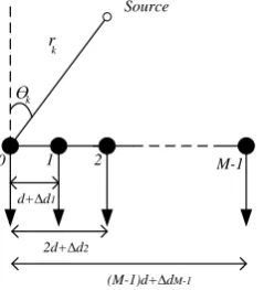
Consider an M element ULA. Sensor at position ‘0’ is taken
as reference sensor and the spacing between the mth sensor and the reference sensor is md+∆dm, m = 1,2,…,M-1 with
perturbation of ∆dm as shown in Fig.1. Suppose that there are K narrow band signals in the near field of ULA. It is assumed that the number of sources is known otherwise it can be
Source
0 1 2 M-1
ϴk rk
d+∆d1
2d+∆d2
(M-1)d+∆dM-1
Figure 1. M element uniform linear array
obtained by using different methods like Akaike Information Theoretic Criteria (AIC) or Minimum Description Length (MDL). The DOAs and ranges of incoming signals are ‘ϴk’
and ‘rk’ respectively where k = 1,2,…,K.
It is assumed that K ≤ M. It is also assumed that the incident signals and noise are uncorrelated. The angles ‘ϴk’ are
estimated w.r.t. the reference sensor. Using Fresnel approximation for near field sources, the signal received at mth
sensor can be written as:
(1) where
with τ0 = 0
In vector form,
(2) where
By using the second-order Taylor series expansion and neglecting the higher order terms, τmk is approximated as
follows:
Thus, the signal received at mth sensor can be re-written as:
; (3) where
and
for k=1,2,… ,K. is the steering vector and n is the additive white Gaussian noise, added to the sensor outputs. Thus, in the presence of array sensor perturbations, the problem under consideration is to estimate the unknown parameters i.e. the angle of arrival ‘θk’ and the range ‘rk’ of
sources, for k=1,2,… ,K and the extent of sensor perturbation
∆dm, from the received data.
3.
METHODOLOGY
DE [10] is taken as the global optimizer in this paper to solve the complex, stochastic, multi-dimension and non-linear objective function, because of its competence in optimization, simplicity in implementation and fast convergence. The procedure is divided into two steps: 1) The sensor position uncertainties are estimated without using any set of calibration sources. 2) DOAs and ranges of near field sources are estimated with sensor position uncertainties estimated in step 1.
3.1
Step 1: Sensor Position Uncertainty
Estimation
First, DOAs and ranges of near-field sources are estimated in the presence of unknown sensor position uncertainties. The initial generation of chromosomes is randomly created.
3.1.1
Initialization
Suppose that L and H are the lower and upper limits of chromosomes respectively. Suppose that the number of chromosomes in a generation is ‘C’ and number of genes on any chromosome is ‘G’, then
(4) where,
c = chromosome number for = gene number for
= generation number`
rand ( ) = a random number chosen from 0 to 1
The chromosome consists of genes in the following order:
After creating the initial generation of chromosomes, the algorithm checks the fitness of all the chromosomes by using:
(5) where,
(6) is the mean square error and ‘ε’ is a very small positive number.
3.1.2
Updating
Update all the chromosomes of the present generation ‘g’ from 1 to C. Suppose we pick up cth chromosome a) Mutation:
Choose three numbers randomly from 1 to C i.e. (c1, c2, c3),
all different and not equal to c. Then use
to create an intermediate chromosome. Here, ‘F’ is the scale
factor (problem dependent) which can be selected from 0.4 to 1.2 but usually selected as 0.5.
b) Crossover:
where, rand ( ) is a number randomly selected from 0 to 1, CR
(cross-over rate) = 0.5 to 0.9 (generally) and is chosen
randomly from 1 to G.
c) Selection: Select the new chromosome by using the following equation i.e. replace the old chromosome with new if the fitness is better.
3.1.3
Termination
If
where,
stop or if the number of generations reached, stop, otherwise go back to updating stage.
These estimated DOAs and ranges are used as calibration parameters to estimate the unknown sensor position uncertainties. The initial generation of chromosomes is randomly created by using eq. (4). The chromosome consists of genes in the following order:
After creating the initial generation of chromosomes, the algorithm checks the fitness of all the chromosomes by using eq. (5). If any of the chromosomes satisfies the condition of termination, the algorithm stops. Otherwise, it goes to the updating stage.
3.2
Step 2: DOA and range estimation with
sensor position uncertainties estimated
in step 1
For this step, the sensor position uncertainties estimated in step 1 are used for the estimation of DOAs and ranges of near-field sources. The algorithm steps are same for DOA and range estimation as in step 1. The summary of proposed methodology is given in Table 1.
4.
NUMERICAL EVALUATION
In this section, MATLAB simulations are presented to verify and discuss the performance of DE algorithm for DOA and range estimation of near field sources in the presence of sensor position uncertainties. A ULA of 10 passive sensors is used. The spacing between two consecutive sensors is taken as λ⁄2 (ideally). The number of sources K is assumed to be known.
Table 1. Summary of the proposed methodology
Given A received signal ‘ ’ from eq. 2 and source number
‘K’.
Step 1 Estimate DOAs and ranges with unknown sensor
position uncertainties
Step 2 Use these estimate DOAs and ranges as calibration
parameters to estimate the unknown sensor position uncertainties.
Step 3 Use the estimated sensor position uncertainties to
estimate the DOAs and ranges of near field sources.
Two near-field sources are assumed to impinge on the ULA with DOAs (30o, 70o) and ranges (20m, 100m). Wavelength λ is taken 2.5m and DE parameters are set as F = 0.4, CR = 0.8 with 50 chromosomes and 300 generations. Noise is added to the sensor outputs and considered as white Gaussian for all cases. The results of DE algorithm are compared with the results of PSO for DOA and range estimation of near field sources in the presence of sensor position uncertainties. The results are averaged over 100 Monte-Carlo simulations.
4.1
4.1 Sensor position uncertainty
estimation
For this step, the actual sensor position uncertainties are set as depicted in Table 2. The DOAs and ranges are estimated in the presence of unknown sensor position uncertainties. Then, these DOAs and ranges are used as calibration parameters and the unknown sensor position uncertainties are estimated. The actual and estimated values of sensor position uncertainties are given in Table 2.
Table 2. Sensor position errors
Sensor number
Ideal position
(m)
Actual position
(m)
∆dm Actual
(m)
∆dm Estimated
(m)
2 2d 2d + ∆d2 0.07 0.0698
5 5d 5d + ∆d5 0.06 0.0594
8 8d 28 + ∆d8 0.08 0.0782
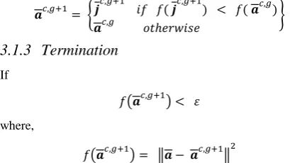
Figure 2. JRMSE of position error estimation vs. Number of Sensors with error
4.2
4.2 DOA and range estimation with
known sensor position uncertainties
4.2.1
Case 1
For this case, SNR is set to 10 dB. The sensor position uncertainties are taken same as estimated in the previous experiment.
Fig. 3 and Fig. 4 plots the JRMSE of DOA and range estimation with different number of sensors with position uncertainties. From Fig. 3 and Fig. 4, it can be seen that the proposed method can accurately estimate the DOAs and ranges of multiple near field sources even when there are multiple array sensors with position uncertainties. It can also be seen that the accuracy of estimation decreases when more array sensors have position uncertainties.
4.2.2
Case 2
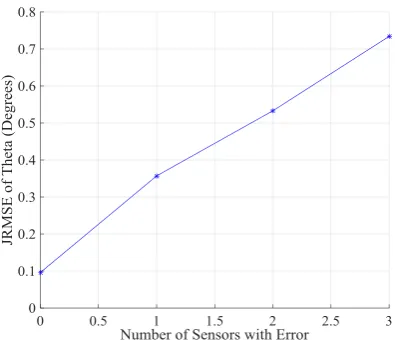
For this case, SNR is changed from -10 dB to 20 dB. The sensor position uncertainties are taken same as estimated in the previous experiment. The results of proposed method are compared with the results of PSO. The swarm size for PSO is taken 110.
Figure 3. JRMSE of DOA estimation vs. number of sensors with error
Figure 4. JRMSE of range estimation vs. number of sensors with error
Figure 6. JRMSE of Range estimation vs. SNR
Fig. 5 and Fig. 6 plots the comparison of performances of DE and PSO for DOA and range estimation of near field sources under two scenarios i) when there are no array sensors with position uncertainties, ii) when there are multiple sensors with position uncertainties. It can be seen from both figures that the proposed method outperforms the method in comparison. The proposed method can perform well even in negative SNRs. It can also be seen that when SNR is lower than -5 dB, the accuracy of DE is effected whereas the error in PSO estimation is unacceptable.
5.
CONCLUSION AND PROSPECTIVE
PLAN
In this paper, the effects of array sensor position uncertainties on near-field source localization for uniform linear arrays have been investigated. DE with MSE as a fitness evaluation function is used because of its ease in employment and single snapshot requirement for convergence. From a large number of Monte-Carlo simulations, it has been demonstrated that DE works eminently even with sensor position uncertainties in terms of robustness to noise and estimation accuracy. The proposed algorithm flops when the number of sensors in the ULA is less than the number of sources as it becomes an underdetermined situation.
The prospective plan is to extend this methodology to near field source localization in the presence of position, gain and phase uncertainties.
6.
REFERENCES
[1] Jinzhou L., Hongwei P., Fucheng G., Le Y. and Wenli J. 2015. Localization of multiple disjoint sources with prior knowledge on source locations in the presence of sensor location errors. Digital Signal Processing. 40 (2015), 181-197.
[2] Sheikh Y. A., Ullah R. and Zhonfu Y. 2016. Range and Direction of Arrival Estimation of Near-Field Sources in Sensor Arrays using Differential Evolution Algorithm. International Journal of Computer Applications (IJCA). Vol. 139 (2016), No.4.
[3] Sun M. and Ho K. C. 2012. Refining inaccurate sensor positions using target at unknown location. Signal Processing. 92 (2012), 2097-2104.
[4] Weiss C. and Zoubir A. M. 2014. Robust High-Resolution DOA Estimation with Array Pre-Calibration. In Proceedings of the 22nd European Signal Processing Conference (EUSIPCO).
[5] Ho K. C., Lu X. and Kovavisaruch L. 2007. Source localization using TDOA and FDOA measurements in the presence of receiver location errors: analysis and solution. IEEE Transactions on Signal Processing. 55 (2007), 684–696.
[6] Yang L. and Ho K. C. 2009. An approximately efficient TDOA localization algorithm in closed-form for locating multiple disjoint sources with erroneous sensor positions. IEEE Transactions on Signal Processing. 57 (2009), 4598–4615.
[7] Lui K. W. K., Ma W. K., So H. C. and Chan F. K. W. 2009. Semidefinite programming approach to sensor network node localization with anchor position uncertainty. In Proceedings of the IEEE International Conference on Acoustics, Speech, and Signal Processing (ICASSP’09).
[8] Chiu W., Chen B. and Yang C. 2011. Robust relative location estimation in wireless sensor networks with inexact position problems. IEEE Transactions on Mobile Computing. 99 (2011) 1.
[9] Sun M. and Ho K. C. 2011. An asymptotically efficient estimator for TDOA and FDOA positioning of multiple disjoint sources in the presence of sensor location uncertainties. IEEE Transactions on Signal Processing. 59 (2011), 3434–3440.
[10] Storn R. and Price K. 1997. Differential Evolution - A Simple and Efficient Heuristic for Global Optimization over Continuous Spaces. Journal of Global optimization. 11 (1997), 341-359.
[11] Nishiura T. and Nakamura S. 2003. Talker localization based on the combination of DOA estimation and statistical sound source identification with microphone array. In proceedings of IEEE Workshop on Statistical Signal Processing.
[12] Zaman F., Qureshi I. M., Naveed A. and Khan Z. U. 2012. Joint Estimation of Amplitude, Direction of Arrival and Range of Near Field Sources using Memetic Computing. Progress In Electromagnetics Research C. 31 (2012), 199-213.
[13] Liang J., Liu D., Zeng X., Wang W., Zhang J. and Chen H. 2011. Joint (azimuth-elevation-range) estimation of mixed near-field and far-field sources using two-stage separated steering vector-based algorithm. Progress In Electromagnetics Research. 113 (2011), 17-46.
[14] Raghu N. C. and Sanyogita S. 1995. Higher-order subspace based algorithms for passive localization of near-field sources. In Proceedings of Twenty-Ninth Asilomar Conference on Signals, Systems and Computers, Pacific Grove, CA.
[15] Huang Y. D. and Barkat M. 1991. Near-field multiple sources localization by passive sensor array. IEEE Trans. Antennas Propag. 39(7) (1991), 968–975.
[17] Abred-Meraim K. and Hua Y. 1998. 3-D near field source localization using second order statistics. In Proceedings of Conf. Record of the 31st Asilomar Conf. on Signals, Systems and Computers, Pacific Grove, CA, USA.
[18] Zaman F., Qureshi I. M., Naveed A. and Khan Z. U. 2012. Real Time Direction of Arrival estimation in Noisy Environment using Particle Swarm Optimization with single snapshot. Research Journal of Engineering and Technology (Maxwell Scientific organization). 4(13) (2012), 1949-1952.
[19] Zaman F., Khan S. U., Ashraf K. and Qureshi I. M. 2014. An Application of Hybrid Differential Evolution to 3-D Near field Source localization. In Proceedings of 2014 11th International Bhurban Conference on Applied Sciences & Technology (IBCAST) Islamabad, Pakistan.
[20] Ao Y. and Chi H. Experimental Study on Differential Evolution Strategies. In Proceedings of Global Congress on Intelligent Systems, IEEE computer society.
[21] Errasti1 B., Escot D., Poyatos D. and Montiel I. 2009. Performance analysis of the Particle Swarm Optimization algorithm when applied to direction of arrival estimation. In Proceedings of ICEAA.
[22] Addad B., Amari S. and Lesage J. J. 2011. Genetic algorithms for delays evaluation in networked automation systems. Engineering Applications of Artificial Intelligence. 24 (2011), 485-490.