FIR Linear Phase Fractional Order Digital Differentiator Design using Convex Optimization

FIR Linear Phase Fractional Order Digital Differentiator

Design using Convex Optimization

Simranjot Singh

Kulbir Singh

ABSTRACT

In this paper, design of linear phase FIR digital differentiators is investigated using convex optimization. The problem of differentiator design is first described in terms of convex optimization with different optimization variables’ options, taken one at a time. The method is then used to design first order low pass differentiators and results are compared with Salesnick’s technique and Parks McClellan algorithm. The designed FIR low pass differentiator has improvement in transition width and flexibility to optimize different parameters. The concept of low pass differentiation is further generalized to fractional order differentiators. Fractional order differentiators are designed by using minmax technique on mean square error. Design examples demonstrate easy design procedure and flexibility in the process as well as improvement over existing fractional order differentiators in terms of mean square error in passband. Finally, fractional order differentiators are designed and used for texture enhancement of color images. Better texture enhancement than existing filtering approaches is established based on average gradient and entropy values.

General Terms

FIR Filter, Fractional order differentiator, Low pass differentiator, Full band differentiator, Image Enhancement.

Keywords

FIR Filter, Fractional order differentiator, Low pass differentiator, Full band differentiator, Image Texture Enhancement.

1.

INTRODUCTION

FIR filters are characterized by following equation

where is input signal and is impulse response. So, they are linear systems described by convolution relation in input and output [1], [2]. Its frequency response is given by

The response can also be written as vector product, as in [3]

The vector and contains real valued filter coefficients. FIR filters have the advantage of linear phase if

filter coefficients are symmetric or anti-symmetric about its center point. The frequency response of linear phase filter can be expressed as

where is amplitude response of the filter, such that

here is half of impulse response and The parameters and depend on length of impulse response and type of FIR linear phase filter [2]. These parameters for the four types of filters are given by

TABLE 1: Properties of the four types of FIR filters

Type I N/2 0

Type II N/2

Type

III N/2 0

Type

IV N/2

(a) (b)

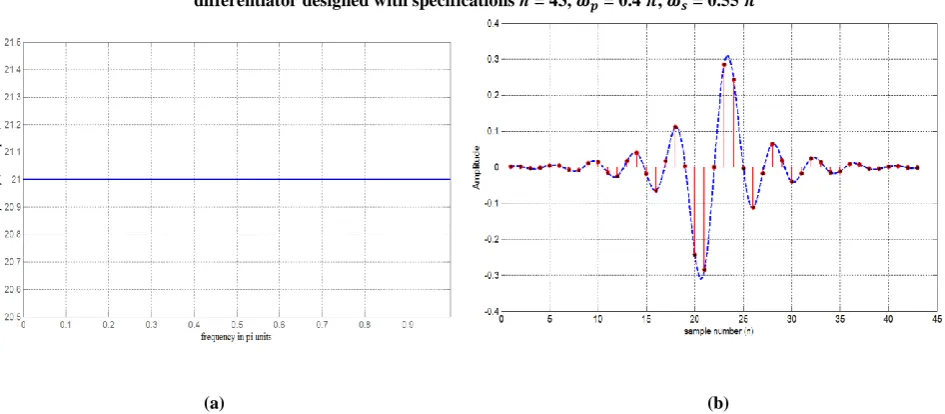
Fig 1 : (a) Magnitude response of differentiator with specifications n = 43, = 0.4 , = 0.55 (b) Error curve of differentiator designed with specifications n = 43, = 0.4 , = 0.55

(a) (b)

Fig 2 : Linear phase of the designed filter in example (a) Group delay introduced by of the design example filter (b) Impulse response of the design example filter

where and are passband and stopband cutoff frequencies respectively.

Optimization design of FIR filters is carried out in two steps [3]. Firstly, characteristic specification by equality or inequality constraints. Then optimal value of a chosen performance metric is calculated using the optimization procedure. The problem can be very difficult to solve but if inequality constraints are convex and equality constraints are affine then any local optimum is global optimum. This highly simplifies the task. Software tools (e.g. [8] and [9]) are available to find global optimum with a little programming, such a MATLAB toolbox we have used in this paper is CVX [8]. Recently, algorithms have been developed that solve convex problems very efficiently [10]. The tools available easily detect infeasibility, arising from inability to solve the problem. FIR filter design problems are convex optimization

problems when symmetry constraints are imposed e.g. in the case of linear phase filter design.

A first order low pass digital differentiator that minimizes passband error ( ) is incorporated here as a design example. This optimization problem can be expressed in terms of spectral mask such that

minimize

subject to + ≤ ≤ - [0, ] ≤ here filter coefficients, , and passband ripple are optimization variables. , , filter order n, stopband attenuation are problem parameters. Passband ripple and stopband attenuation can also be expressed in decibels i.e. as

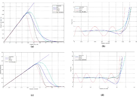
(a) (b)

(c) (d)

Fig 3 : Magnitude and error plots of convex, Salesnick’s, Parks-McClellan and Alaoui’s techniques (a) Magnitude response for = 0.35 (b) Error curves for = 0.35 (c) Magnitude response for = 0.52 (d) Error curves for = 0.52 taken as 50 dB. No constraints are imposed on magnitude

response in transition region. If the problem is feasible and can be solved, then half of the impulse response ( ) is obtained. The end part of methodology is changing the impulse response to an anti-symmetric form, so that the designed filter has linear phase. Magnitude response of the filter is plotted in Figure 1(a). Impulse response is shown in Figure 2(b), constant group delay of the filter designed can be seen in Figure 2(a). As the transfer function of the designed filter in -domain is

The error, plotted in Figure 1(b), is difference between magnitude response and ideal response. Error graph provides insight into passband performance of the filter, it can also be produced in terms of percentage (%age) error [12], which is equal to . The above mask problem formulation contains semi-infinite inequality constraints [11]. These can be approximated by using frequency sampling. It is done by taking a set of frequencies in [0, ], i.e.

or [ ] as required. Then we can replace semi-infinite inequality constraints with N inequality constraints because sampling preserves convexity [11]. N = 30 n is taken here to design the filters. Frequency band of approximation depends

on problem and frequency region of response of the filter. For example, we have used approximation in both passband and stopband for spectral mask filter design case. For MSE minmax design scenario, discussed later in the chapter, the approximation is taken upto a particular point in passband frequency range (enhancing filter response in that particular region).

2.

LOW PASS DIFFERENTIATORS

The design process of low pass differentiators can be categorized into three parts, such that the differentiator is designed for given specifications. In the following sections linear phase FIR type III digital differentiators are designed for first order case.

2.1

Differentiator design with minimum

passband error

This convex problem is same as that we have discussed in detail in formulation (7).

2.2

Differentiator design with minimum

transition width

are important for suppression of high frequency noise.

2.3

Differentiator design with minimum

order

n

In this case, available maximum order of the differentiator is provided and then an optimization procedure could be used to find minimum order of the filter. By solving the feasibility problems, filter length can be minimized. The feasibility check consists of same constraints as in (7), with passband ripple fixed. An optimization algorithm can be utilized to achieve minimum of n. For example, an efficient solution is bisection on n.

We can also pose the problem to design low pass differentiators as minmax formulation on mean square error minimize

subject to ≤ The same options discussed in the design of first order case can also be taken, similarly, in higher order differentiators.

3.

FRACTIONAL ORDER

DIFFERENTIATOR

In this section, type IV fractional order digital differentiators are designed. To evaluate performance and compare different methods the integral squares error of frequency response is used

To exploit above relation, minmax technique is applied on

_{. Therefore the unconstrained convex} optimization problem [14] can be stated as

minimize

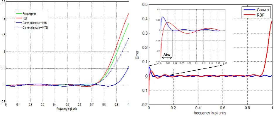
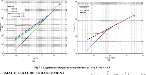
is illustrated in Figure 4(a). The differentiator order equals 1.5, designed in [15], and plotted in Figure 4(b). Comparison illustration using error plots is done in Figure 5(a), it is observed that error in case of = 0.72 is much less than =

0.9 case, so that by varying we can control inband accuracy. In [14], the differentiator was designed by minimizing error

up to 0.72 , however here we can easily minimize error with an option to vary the differentiator bandwidth. for different values of of these three of the methods are given in Table II. Magnitude response of fractional differentiator for λ = 0.9 is shown in Figure 4(b). Hence frequency response is more easily and accurately approximated by convex optimization technique.

Another fractional order differentiator is designed with v = 0.5. The design specifications are n = 60, v = 0.5, = . In [7], authors have produced improved fractional order differentiator, using RBF, with respect to fractional delay method. In this design example same method is compared with RBF technique with specifications n = 61, I = 20, v =

0.5, h = 0.1, L = 620 and Gaussian RBF with σ = 2.3. Error of RBF fractional order differentiator, for = 1, is 4.1 x and error of convex optimization method is 6.04 x . The response the designed filters are shown in Figure 6, along with log-log plot in Figure 7, for more better graphical presentation of response at low frequency (especially near transition width). There are certain points to be taken care of such as slope of ideal differentiator’s frequency response at

is infinity so some transition width should be provided at the point. This width is illustrated in Figure 6(b), the error plot, it is denoted by Δtw in the graph, in this example it is taken 0.03 . Differentiator designed in [7] need modification in coefficients because of the non-zero gain at , however in this method, the design process is simpler and no requirement of such modifications.

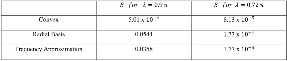
Table II. comparison of Convex Optimization, Radial Basis and Frequency Approximation based design for λ = 0.72 and 0.9

Convex

5.01 x

8.13 x

Radial Basis

0.0544

1.77 x

(c) (d)

Fig 5 : (a) Error plot for first fractional order differentiator design (v = 1.5) with convex optimization, RBF, frequency approximation method (b) Error graphs for second filter design (v = 0.5) using convex optimization and RBF

(a) (b)

(a) (b) Fig 7 : Logarithmic magnitude response for (a) v=1.5 (b) v = 0.5

4.

IMAGE TEXTURE ENHANCEMENT

Image sharpening is a very useful image processing tool. It is used in many applications from medical imaging to artificial intelligence [7]. Texture enhancement is needed due to blurring of the picture. Image sharpening is implemented in [7] by generalizing the concept of Laplacian method to fraction values. The same technique is used here to demonstrate the use of designed novel fractional order differentiator, comparison can be done by assessing the quality of images. The enhancement of the images can be measured using parameters like average gradient and entropy [15]. Greater average gradient means clearer image and greater entropy shows that the image has greater texture details [16], [17]. Their higher value for the processed image, for same fractional order (v), depicts more efficient system. Average gradient and entropy for a grayscale image, with dimensions P X , are defined as follows

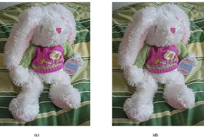
The schematic shown in Figure 8 is implemented in MATLAB by forward and backward filtering approach. Each plane (R, G and B) is passed through the filter independently and added to original image and gradient images. Average gradient and entropy are calculated for color images by taking mean of the three planes (R, G and B). The order of differentiation needed for same amount of image sharpening is relatively less in case of convex optimization based design as compared to RBF approach. The parameters for designed type IV differentiator are n = 6, = 1. The realization of implementation is shown in Figure 8. f (x,y) is the original image and p (x,y) is enhanced image. Some example images taken from [18] are demonstrated in Figure 9 and Figure 10. Comparison of Convex Optimization and Radial Basis Function (RBF) based designed fractional order digital differentiators using average gradient and entropy is done in Table III. As it can be seen by the statistics convex optimization based filter implementation proves to be better image enhancement technique.

.

(a)

(b)

(c)

(d)

Fig 9 : Dandelion image and enhanced images using various order of differentiation. (a) Original image (b) v = 0.4 (c) v = 0.8 (d) v = 1.2

(a)

(c)

(d)

Fig 10 : Rabbit image and enhanced images using various order of differentiation. (a) Original image (b) v = 0.4 (c) v = 0.8 (d) v

= 1.2

Table III. Image enhancement comparison using Average Gradient and entropy of Radial Basis Function, Convex Optimization based designs

Fractional

Order (v)

Rabbit

Dandeli

Average Gradient

Entropy

Average

Gradient

Entropy

Convex

RBF

Convex

RBF

Convex

RBF

Convex

RBF

0.4

12.844

12.2122

7.755

7.693

9.799

9.341

7.186

7.197

0.8

14.084

11.982

7.741

7.699

11.434

9.297

7.218

7.192

1.2

18.98

15.21

7.7464

7.337

16.488

12.211

7.26

7.22

5.

CONCLUSIONS

The paper describes the design of linear phase digital differentiators using convex optimization technique. It is shown that various types of differentiator design problems can be formulated as convex semi-infinite problems. It is observed that the approach is very easy and gives us the flexibility to optimize desired parameter of the system. The method is then used to design first order low pass differentiators, we have discussed different options available separately. It is illustrated that the designed differentiator has less transition width and overshoot in frequency response, as compared to other techniques, [5] and [6]. The problem of fractional order

Magazine.

[4] Roy, S.C.D. and Kumar, B. 1993. Handbook of Statistics. Vol. 10. Elsevier Science Publishers. Amsterdam. pp.159-205.

[5] Tseng, C.C. and Lee, S.L. 2006. Linear phase FIR differentiator design based on maximum signal-to-noise ratio criterion. Signal Processing. vol. 86.

[6] Salesnick, I. 2002. Maximally flat lowpass digital differentiators. IEEE Trans. Circuits Syst. II. vol. 49. no. 3. pp. 219–223.

[7] Tseng, C.C. and Lee, S.L.. 2008. Design of Fractional Order Digital Differentiator Using Radial Basis Function. IEEE Transactions On Circuits And Systems—I: Regular Papers. Vol. 57. No. 7

[8] Grant, M., Boyd S.: Graph implementations for nonsmooth convex programs. Recent Advances in Learning and Control, V. Blondel, S. Boyd, and H. Kimura, Eds. New York: Springer, pp. 95–110 [Online]. Available: http://stanford.edu/ ˜boyd/cvx (2008)

[9] Sturm, J. F. 1999. 1999. Using SeDuMi 1.02, a Matlab toolbox for optimization over symmetric cones. Optim. Methods and Software vol. 11–12. pp. 625–653. [Online] Available: http://sedumi.ie.lehigh.edu

Physiological Signal Processing. CSNDSP 2010,.pp. 747 – 750

[14] Boyd, S. and Vandenberghe L.2004. Convex Optimization. Cambridge Univ. Press, Cambridge. U.K. [15] Zhao, H., Qiu G., Yao L. and Yu, J..2005. Design of

fractional order digital FIR differentiators using frequency response approximation. Proc. 2005 Int. Conf. Communications, Circuits and Systems. pp. 1318–1321. [16] Yakhdani, M. F. and Azizi, A. 2010. Quality Assessment

of Image Fusion Techniques For Multisensor High Resolution Satellite Images. The International Archives of Photogrammetry, Remote Sensing and Spatial Information Sciences. Vol. 38. Part 7B. pp. 204-209 [17] Hao, M. and Sun, X.. A modified Retinex Algorithm

based on Wavelet Transformation. Second International Conference on MultiMedia and Information Technology 2010. pp. 306-309

[18] Garg, V. and Singh, K. . 2012. An Improved Grunwald-Letnikov Fractional Differential Mask for Image Texture Enhancement, International Journal of Advanced Computer Science and Applications. vol. 3. no. 3. [19] Levin A., Lischinski D. and Weiss, Y. 2008 .A