Application of Thunderstorm Algorithm for Defining the Committed Power Output Considered Cloud Charges

(1)

International Journal of Advanced Engineering, Management and Science (IJAEMS) [Vol-2, Issue-5, May- 2016] Infogain Publication (Infogainpublication.com) ISSN : 2454-1311

www.ijaems.com Page | 293

Application of Thunderstorm Algorithm for

Defining the Committed Power Output

Considered Cloud Charges

A.N. Afandi

Electrical Engineering, Universitas Negeri Malang, Indonesia

Abstract— This paper presents an application of

Thunderstorm Algorithm for determining a committed power output considered cloud charges with various technical constraints and an environmental requirement. These works also implemented on IEEE-62 bus system throughout an operational economic dispatch covered for economic and emission aspects. The results obtained show that statistical and numerical performances are associated with charges. It also presents fast and stable characteristics for the searching speeds. By considering

the cloud charge parameter, it contributes to

performances and results of Thunderstorm Algorithm. In addition, the introduced algorithm seems strongly to be a new promising approach for defining the committed power output problem.

Keywords—Cloud charge, economic dispatch, intelligent computation, power system, thunderstorm algorithm.

I. INTRODUCTION

Presently, technical problems are more complicated than previous cases included numerous variables for representing physical systems in suitable models as closed as its functions in nature with natural characteristics and behaviours. Many problems have become crucial topics to solve correctly in feasible ranges within high qualities under numerous constraints and environmental requirements for searching the desired performances. To cover these conditions, the problems adopted many parameters are expressed in optimization functions considered potential variables and limitations in order to obtain better solutions within a period time operation. Moreover, these functions are conducted to designed models for presenting real cases in mathematical statements as the objective function constrined by technical conditions and environmental requirements.

By considering mathematical expressions, real problems are solvable easily using various methods of computations associated with its defined functions through traditional or evolutionary approaches. Both

methods are commonly used to carry out the problem and applied to evaluate its performances. Actually, these approaches has different characteristics while searching the optimal solution. In detail, traditional methods use mathematical programs given in various versions as the proposed names at the early introduction. As long as the period implementation, popular classical methods are linear programming, lambda iteration, quadratic programming, gradient search, Newton’s method, dynamic programming, and Lagrangian relaxation [1], [2], [3], [4]. On the other hand, evolutionary methods use optimization techniques, such as genetic algorithm, neural network, simulated annealing, evolutionary programming, ant colony algorithm, particle swarm optimization, and harvest season artificial bee colony algorthm [5], [6], [7], [8], [9]. These methods have been proposed for replacing classical approaches on the base of its weaknesses considered many phenomena and behaviours in nature with mimicking its mechanisms. Nowadays, evolutionary methods are frequently used to solve optimization problems, not only for real cases but also for designed themes [10]. These methods are useful for breaking out large systems and multi dimensions constructued using multiple variables and constraints. In particular, many types have been proposed at different times as an introduction early based on its inspirations. Since the first time of the evolutionary idea became a new computation era out of the classical period, many works have been done for developing and improving its performances with modified techniques and phases. Moreover, these developments are also subjected to expand computational performances for increasing abilities to carry out numerous problems with many proposed procedures.

(2)

www.ijaems.com Page | 294 II. THUNDERSTORM ALGORITHM

At present, the lightning is considered as an atmospheric discharge during thunderstorms or other possibility factors produced by several steps in terms of Charge separation; Leader formation; and Discharge channel. Moreover, the lightning process is defined as an electric discharge in the form of a spark in a charged cloud that the negative and positive charges are deployed at different positions [11], [12], [13]. In addition, a seat of electrical processes can be produced by a thunderstorm and it is rapidly advanced during the continuous lightning in the thunderstorm. In this phenomenon, the defining atmospheric material for the thunderstorm is very important things and urgently observations covered in moisture; unstable air; and lift.

Many studies have been done to observe these phenomena with numerous discussions for searching suitable models and understanding its mechanisms. Various characteristics have been tested and reported for analyzing these curious issues in many studies in order to recognize natural behaviours [14], [15], [16], [11], [12], [17], [18], [19], [20]. In general, the introduced algorithm entitled Thunderstorm Algorithm (TA) has adopted a phenomenon in nature for pretending natural processes performed using several stages to explain the adoption of the inspiration [21]. Furthermore, this inspiration is associated with a natural mechanism conducted to define multiple natural lightning in the computation.

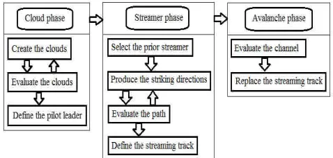
Fig. 1: Thunderstorm Algorithm’s Phases

By considering this phenomenon, its mechanisms are transferred into certain procedures as the sequencing computation presented in pseudo-codes in terms of Cloud Phase; Streamer Phase; and Avalanche Phase [21]. Cloud Phase is used to produce cloud charges and to evaluate the clouds before defining the pilot leader. Another step, Streamer Phase, is supposed to define the prior streamer and to guide striking directions included the path evaluation for defining the streaming track. The final process is Avalanche Phase, which is used to evaluate channels, replace the streaming track for keeping the streamer. In detail, these phases are depicted in Fig. 1.

In these phases, the searching mechanism is conducted to striking processes and channeling avalanches to deploy the cloud charges, which is populated using (1). Moreover, TA is also consisted of various distances of the striking direction related to the hazardous factor for each position of the striking targets as presented in (2). Each solution is located randomly based on the generating random directions of multiple striking targets. In principle, the sequencing computation of TA is given in several procedures as presented in following mathematical main functions.

Cloud charge: Q = (1 + k. c). Q , (1)

Striking path: D = (Q ).b.k, (2)

Charge’s probability: probQ_sj Q_sjm

∑Q_smfor m Q_sjn

∑Q_sn for n

, (3)

where Qsj is the current charge, Qmidj is the middle charges, s is the streaming flow, Dsj is the striking charge’s position, Qsdep is the deployed distance, n is the striking direction of the hth, k is the random number with [-1 and 1], c is the random within [1 and h], h is the hazardous factor, b is the random within (1-a), n is the striking direction, j ∈ (1,2,..,a), a is the number of variables, m ∈ (1,2,..,h).

III. COMMITTED POWER OUTPUT

The power system operation is able to measure using a financial aspect for defining the whole operation, such as fixed cost; maintenance cost; and production cost, in order to the PSOP can be conditioned in an economic portion with the suitable budget. Since the operation is concerned in the technical cost of products and services, the optimal operation and planning are very important things for deciding in the balanced power production. Economically, these problems become urgently issues to decrease running charges of the electric energy while supplying load demands at different places. It also needs to manage using an economic strategy for selecting the optimal operating cost.

(3)

www.ijaems.com Page | 295 dispatch (ED) [23], [24], [26]. Moreover, The IED is

formulated by equation (4) and each fuel cost participation is expressed in (5) for defining the LD as given in (6). In particular, the individual pollutant discharge of generating unit is formed in (7) and the ED’s function is presented in (8) for all participants in the CPO. In general, the CPO is commonly approached using main mathematical functions as follows:

IED: _Φ= w. F + (1 − w). h. E , (4) Fi(Pi) =ci+biPi +aiPi2 , (5)

LD: F = ∑ (c + b . P + a . P_#$" !), (6)

E (P) = γ +β. P +α. P!, (7)

ED: E = ∑ &_#$" γ +β. P +α. P!', (8)

where Φ is the IED ($/h), w is a compromised factor, h is a penalty factor, Ftc is the total fuel cost ($/h), Et is the total emission (kg/h), Fi is the fuel cost of the ith generating unit ($/h), Pi is a power output of the ith generating unit, ai; bi; ci are fuel cost coefficients of the ith generating unit, ng is the number of generating unit, Ei is an emission of the ith generating unit (kg/h), αi; βi; γi are emission coefficients of the ith generating unit.

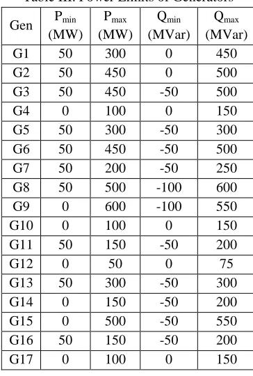
IV. APPLICATION’S PROCEDURES In these studies, simulations adopt a standard model of the power system for demonstrating the impact of the cloud charges related to the CPO with various technical constraints. The use of the standard model is commonly approached by researchers for performing own problems, even practical systems are also able to apply for the same problem. In these works, the IEEE-62 bus system is selected as the sample system, which is consisted of 19 generators; 62 buses; and 89 lines as discussed completely in [24]. Technically, it data are presented in Table I; Table II; and Table III for coefficients and power limits which are given in individual generating units.

Table I. Fuel Cost Coefficients

Gen α β γ Gen α β γ

G1 0.0070 6.80 95 G11 0.00450 1.60 65 G2 0.0055 4.00 30 G12 0.00250 0.85 78 G3 0.0055 4.00 45 G13 0.00500 1.80 75 G4 0.0025 0.85 10 G14 0.00450 1.60 85 G5 0.0060 4.60 20 G15 0.00650 4.70 80 G6 0.0055 4.00 90 G16 0.00450 1.40 90 G7 0.0065 4.70 42 G17 0.00250 0.85 10 G8 0.0075 5.00 46 G18 0.00450 1.60 25 G9 0.0085 6.00 55 G19 0.00800 5.50 90 G10 0.0020 0.50 58 a ($/MWh2), b ($/MWh)

Table II. Emission Coefficients Ge

n a b c

Ge

n a b c

G1 0.01 8 -1.8 1 24.3 0 G1 1 0.01 4 -1.2 5 23.0 1

G2 0.03 3 -2.5 0 27.0 2 G1 2 0.01 2 -1.2 7 21.0 9

G3 0.03 3 -2.5 0 27.0 2 G1 3 0.01 8 -1.8 1 24.3 0

G4 0.01 4 -1.3 0 22.0 7 G1 4 0.01 4 -1.2 0 23.0 6

G5 0.01 8 -1.8 1 24.3 0 G1 5 0.03 6 -3.0 0 29.0 0

G6 0.03 3 -2.5 0 27.0 2 G1 6 0.01 4 -1.2 5 23.0 1

G7 0.01 3 -1.3 6 23.0 4 G1 7 0.01 4 -1.3 0 22.0 7

G8 0.03 6 -3.0 0 29.0 3 G1 8 0.01 8 -1.8 1 24.3 0

G9 0.04 0 -3.2 0 27.0 5 G1 9 0.04 0 -3.0 0 27.0 1 G1 0 0.01 4 -1.3 0 22.0 7

α (kg/MWh2), β (kg/MWh)

Table III. Power Limits of Generators

Gen Pmin (MW) Pmax (MW) Qmin (MVar) Qmax (MVar)

G1 50 300 0 450

G2 50 450 0 500

G3 50 450 -50 500

G4 0 100 0 150

G5 50 300 -50 300 G6 50 450 -50 500 G7 50 200 -50 250 G8 50 500 -100 600 G9 0 600 -100 550

G10 0 100 0 150

G11 50 150 -50 200

G12 0 50 0 75

G13 50 300 -50 300 G14 0 150 -50 200 G15 0 500 -50 550 G16 50 150 -50 200

(4)

International Journal of Advanced Engineering, Management and Science (IJAEMS) Infogain Publication (Infogainpublication.com

www.ijaems.com G18 50 300 -50

G19 100 600 -100

These applications are applied to IEEE-62 bus system as the power system model using several programs, which are compiled together in the sequencing processes based on the pseudo-codes covered the cloud phase; streamer phase; and avalanche phase. Each phase follows its mechanism for involving all parameters of TA in the processes while searching the optimal solution with various charges in the cloud charge phase.

In particular, these processes are run in designed programs in terms of main program; evaluate program; cloud charge program; streamer program; avalanche program; and dead track program. N addition, TA performed using 1 of the avalanche; 100 of the streaming flows; and 4 of the hazardous factor. Moreover, the tested system feeds the power production for 2,766.7 MW and 1,206.1 MVar of load demands constrained by 10% of the total loss; 0.5 of the weighting factor; 0.85 kg/h of the standard emission; ± 5% of voltage violations at each bus; and 95% of the power transfer capability for the line.

V. RESULTS AND DISCUSSIONS

As given in the previous section, these works consider 2,766.7 MW for the load constrained by various technical limitations. By considering 10% of the total loss; 0.85 kg/h of the standard emission; the equilibrium

demand and the power production, the cloud charge distributions are illustrated in following

figures are presented for each cloud size

and 100 charges, which are deployed at different positions randomly in Fig. 2; Fig. 3; Fig. 4; and Fig.

to these figures, charges affect to the cloud’s characteristics and charged density within

desired locations. In detail, the highest size has the highest density for the charge.

Fig. 2: Cloud’s profile with 25 charges

International Journal of Advanced Engineering, Management and Science (IJAEMS) Infogainpublication.com)

400

600

62 bus system as the power system model using several programs, which are compiled together in the sequencing processes based codes covered the cloud phase; streamer phase; and avalanche phase. Each phase follows its for involving all parameters of TA in the processes while searching the optimal solution with

hese processes are run in designed programs in terms of main program; evaluate program; rogram; streamer program; avalanche N addition, TA is performed using 1 of the avalanche; 100 of the streaming flows; and 4 of the hazardous factor. Moreover, the tested system feeds the power production for 2,766.7 MW and 1,206.1 MVar of load demands constrained by 10% of the total loss; 0.5 of the weighting factor; 0.85 kg/h of the 5% of voltage violations at each bus; and 95% of the power transfer capability for the line.

DISCUSSIONS

As given in the previous section, these works consider 2,766.7 MW for the load constrained by various technical 10% of the total loss; 0.85 equilibrium of the load on, the cloud charge distributions are illustrated in following figures. These s are presented for each cloud size for 25; 50; 75; and 100 charges, which are deployed at different positions Fig. 5. According s, charges affect to the cloud’s within different desired locations. In detail, the highest size has the

Cloud’s profile with 25 charges

Table IV. Statistical Results Based on N

o Parameters 25

1 Max point ($/h)

17,15 1

2 Min point ($/h)

16,72 0 3 Range ($/h) 431

4 Mean ($/h) 16,75 1

5 Median ($/h) 16,72 0

[Vol-2, Issue-5, May- 2016] ISSN : 2454-1311

Page | 296

Table IV. Statistical Results Based on the Charges Cloud charges

50 75 100 17,15 16,63

3

17,66 6

16,53 9 16,72 16,12

0

16,45 5

15,84 1 431 513 1,211 698 16,75 16,18

7

16,61 3

15,91 5 16,72 16,12

0

16,45 5

(5)

International Journal of Advanced Engineering, Management and Science (IJAEMS) Infogain Publication (Infogainpublication.com

www.ijaems.com 6 Streaming 14 19

7 Opt. time (s) 2.6 3.5 8 Run time (s) 16.9 17.2 Graphically, TA’s abilities are give in Fig.

for streaming flows and time consumptions associated with cloud charges. Fig. 6 presents convergence speeds of computations while finishing all processes for determining optimal solutions in 100 streaming flows with its individual time usage for each process as illustrated in Fig. 7. Moreover, the processes have different started points for searching solutions of the as similar as the obtained streaming flows of the optimal points remained in different speeds. For 25 charges, the computation is started at 17,151 $/h before declining to 16,720 for the optimal position obtained in

consuming 2.6 s of the running time. This execution needs around 16.9 s for completing 100 of the streaming flow. In general, the solution is searched in smooth and fast even the cloud charges used different amounts. In detail, its statistical performances are listed in Table IV covered in maximum points; minimum points; range; and median.

Furthermore, various time consumptions are depicted in Fig. 7 related to cloud charges. This figure

random time consumptions, which are used to search the optimal solutions and to complete the processes of the IED problem considered LD and ED. By considering these compilations, all results are also provided in Table IV for the optimal time usage and the running time for streaming flows. According to these results, the higher cloud size has longer time consumptions, which are 6.2 s for obtaining the solution and 18.8 s for completing the computation associated with 100 of charges.

Fig. 6: Convergences considered the charges

International Journal of Advanced Engineering, Management and Science (IJAEMS) Infogainpublication.com)

25 30

5.6 6.2 18.5 18.8 Fig. 6 and Fig. 7 for streaming flows and time consumptions associated 6 presents convergence speeds of computations while finishing all processes for determining optimal solutions in 100 streaming flows with its individual time usage for each process as 7. Moreover, the processes have oints for searching solutions of the IED as similar as the obtained streaming flows of the optimal points remained in different speeds. For 25 charges, the computation is started at 17,151 $/h before declining to 16,720 for the optimal position obtained in 14 steps with consuming 2.6 s of the running time. This execution also needs around 16.9 s for completing 100 of the streaming flow. In general, the solution is searched in smooth and fast even the cloud charges used different amounts. In tistical performances are listed in Table IV maximum points; minimum points; range; and

, various time consumptions are depicted in figure illustrates the re used to search the optimal solutions and to complete the processes of the problem considered LD and ED. By considering these compilations, all results are also provided in Table IV for the optimal time usage and the running time for According to these results, the higher cloud size has longer time consumptions, which are 6.2 s for obtaining the solution and 18.8 s for completing the computation associated with 100 of charges.

considered the charges

Fig. 7: Time consumptions considered the charges

Table V. Power Productions Based on the Charges

Gen Power outputs (MW) 25 50

G1 105.7 105.7 G2 200.0 265.7 G3 227.2 78.4 G4 99.6 91.9 G5 294.2 105.7 G6) 395.9 395.2 G7 108.6 108.6 G8 234.9 227.7 G9 87.9 273.6 G10 91.9 91.9 G11 80.1 147.2 G12 105.3 105.3 G13 149.3 287.8 G14 137.0 150.0 G15 90.2 90.2 G16 149.6 104.6 G17 91.9 91.9 G18 105.8 200.8 G19 240.7 100.0 Total 2,995.8 3,022.1 Load 2,766.7 2,766.7 Loss 229.1 255.4

Refer to multiple directions as presented as the hazardous factor in TA’s processes, all numerous statistical results are provided in Table IV associated with cloud charges as depicted in Fig. 2 to Fig. 5 for the cloud charge’s profiles. In addition, Table IV has been performed by each procedure of TA while determining optimal solutions to meet 2,776.7 MW of the load. This table shows that the cloud charges give impacts on various aspects, such as, maximum points; optimal points; and times

[Vol-2, Issue-5, May- 2016] ISSN : 2454-1311

Page | 297

Time consumptions considered the charges

Table V. Power Productions Based on the Charges Power outputs (MW)

50 75 100 105.7 105.7 105.7 265.7 376.6 343.4 78.4 132.1 78.4 91.9 93.1 91.9 105.7 190.7 174.6 395.2 291.0 186.1 108.6 166.3 108.6 227.7 278.8 266.2 273.6 87.9 239.0 91.9 91.9 91.9 147.2 149.1 83.5 105.3 105.3 105.3 287.8 105.7 252.7 150.0 70.8 146.9 90.2 99.6 90.2 104.6 104.6 150.0

91.9 91.9 91.9 200.8 270.3 292.8 100.0 210.5 100.0 3,022.1 3,021.9 2,999.0 2,766.7 2,766.7 2,766.7 255.4 255.2 232.3 Refer to multiple directions as presented as the hazardous factor in TA’s processes, all numerous statistical results are provided in Table IV associated with cloud charges as 5 for the cloud charge’s profiles. IV has been performed by each procedure of TA while determining optimal solutions to meet 2,776.7 MW of the load. This table shows that the cloud charges give impacts on various aspects, such as,

(6)

www.ijaems.com Page | 298 Table VI. Emissions Based on the Charges

Gen Pollution productions (kg/h)

25 50 75 100

G1 34.1 34.1 34.1 34.1 G2 847.2 1,692.3 3,765.9 3,059.3 G3 1,162.8 33.9 272.6 33.9 G4 31.5 20.8 22.4 20.8 G5 1,049.9 34.1 333.5 257.0 G6) 4,209.8 4,193.0 2,093.8 704.3 G7 28.7 28.7 156.5 28.7 G8 1,310.2 1,211.9 1,991.3 1,782.1 G9 54.8 2,146.3 54.8 1,547.6 G10 20.8 20.8 20.8 20.8 G11 12.7 142.4 147.7 16.2 G12 20.4 20.4 20.4 20.4 G13 155.1 994.4 34.1 716.1 G14 121.5 158.1 8.3 148.9 G15 51.3 51.3 87.4 51.3 G16 149.2 45.4 45.4 150.5 G17 20.8 20.8 20.8 20.8 G18 34.3 386.4 850.4 1,037.2 G19 1,622.8 127.0 1,167.5 127.0 Total 10,938.0 11,362.2 11,127.8 9,777.0

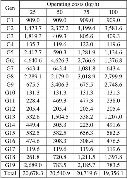
Table VII. Operational Fees Based on the Charges

Gen Operating costs (kg/h)

25 50 75 100

G1 909.0 909.0 909.0 909.0 G2 1,473.7 2,327.2 4,199.4 3,581.6 G3 1,819.3 409.3 805.6 409.3 G4 135.3 119.6 122.0 119.6 G5 2,417.7 590.3 1,281.9 1,134.6 G6) 4,640.6 4,626.3 2,766.6 1,376.8 G7 643.4 643.4 1,081.8 643.4 G8 2,289.1 2,179.0 3,018.9 2,799.9 G9 675.5 3,406.3 675.5 2,748.6 G10 131.3 131.3 131.3 131.3 G11 228.4 469.3 477.3 238.0 G12 205.4 205.4 205.4 205.4 G13 532.6 1,504.5 338.2 1,207.0 G14 449.4 505.3 225.0 491.6 G15 582.5 582.5 656.3 582.5 G16 474.6 308.3 308.4 476.5 G17 119.6 119.6 119.6 119.6 G18 261.8 720.8 1,211.5 1,397.8 G19 2,689.0 783.5 2,185.7 783.5 Total 20,678.3 20,540.9 20,719.6 19,356.1

Final results of the PSOP based on the CPO are presented in the IED as provided in Table V covered cloud charges for the individual power production. This table also

provides the committed power output and the total loss to meet the load. According to this table, it is known that generating units contribute to the power procurement with different capacities as own scheduled power productions. Its pollutant productions are listed in Table VI for 19 generating units. Specifically G10 feeds to the power to the system in the constant amount of 91.9 MW. This condition is also given by G1 and G17 produced in 105.7 MW and 91.9 MW. In total, generating units deliver the power to the load center from 2,995.8 MW to 3,022.1 MW with various amounts of the power loss related to the each cloud charge as given in Table V. As the impact of the environmental requirement, these power productions also discharge pollutants around 9,777.0 kg/h to 11,362.2 kg/h corresponded to cloud charges with individual contributions for the emissions as given in Table VI. In detail, the higher pollutant contributors are G2; G3; G5; G6; G8; and G19.

By considering the whole selections for determining the optimal solutions of the IED problem, the cheapest operation is determined using the higher cloud charge as provided in Table VII presented totally for fuel costs and emission cost compensations. This operation needs around 19,356.1 $ for existing generating units during producing power outputs to meet the load demand. In accordance to individual power productions, several generators spent the budget in high procurement. Practically, power outputs of generating units are associated with the load to set fixed power outputs. The least operating cost becomes a very crucial decision for operating the system in the cheapest budget. In this case, the expensive operations are belonged to several generating units while producing powers, such as, G2; G3; G5; G6; and G19, even these payments are depended on cloud charges. For all compositions of cloud charges, the cheapest operation is existed by G17 with spent in 119.6 $/h.

VI. CONCLUSIONS

(7)

www.ijaems.com Page | 299 REFERENCES

[1] A.A. El-Keib, H.Ma, and J.L. Hart, “Environmentally Constrained ED using the Lagrangian Relaxation Method,” IEEE transactions on Power Systems, vol. 9, pp. 533-534, November 1994.

[2] Ahmed Farag, Samir Al-Baiyat, T.C. Cheng, “Economic Load Dispatch Multiobjective Optimization Procedures using Linear Programming Techniques,”. IEEE Transactions on Power Systems, vol. 10, pp. 731-738, October 1995.

[3] Jose Luis Martines Ramos, Alicia Troncoso Lora, Jesus Riquelme Santos, Antonio Gomez Exposito, “Short Term Hydro Thermal Coordination Based on Interior Point Nonlinear Programming and Genetic Algorithms,” IEEE Porto Power Tech Conference, Potugal, September 2001.

[4] Yong Fu, Mohammad Shahidehpour, Zuyi Li, “Security Constrained Unit Commitment with AC Constraints,” IEEE Transactions on Power Systems, vol. 20, pp. 1538-1550, August 2005.

[5] John G. Vlachogiannis, Kwang Y. Lee, “Quantum-Inspired Evolutionary Algorithm for Real and Reactive Power Dispatch,” IEEE Transactions on Power Systems, vol. 23, pp. 1627-1636, November 2008.

[6] M.A. Abido, “Environtment/Economic Power Dispatch using Multiobjective Evolutionary Algorithms,” IEEE Transactions on Power System, vol. 18, pp. 1529-1539, November 2003.

[7] A.N. Afandi, Hajime Miyauchi, “Solving combined economic and emission dispatch using harvest season artificial bee colony algorithm considering food source placements and modified rates,” International Journal on Electrical Engineering and Informatics, vol. 9, pp. 266-279, Juni 2014.

[8] M.A. Abido, “Multiobjective Evolutionary Algorithms for Electric Power Dispatch Problem,” IEEE Transactions on Evolutionary Computation, vol. 10, pp. 315-329, June 2006.

[9] Z.-L. Gaing, “Particle Swarm Optimization to Solving the ED Considering the Generator Constraints,” IEEE Trans. Power Systems, vol. 18, pp. 1187-1195, August 2003.

[10] A.N. Afandi, Hajime Miyauchi, “Improved Artificial Bee Colony Algorithm Considering Harvest Season for Computing Economic Disatch on Power System,” IEEJ Transactions on Electrical and Electronic Engineering, vol. 9, pp. 251-257, May 2014.

[11] T. J. Lang, S. A. Rutledge, and K. C. Wiens, “Origins of Positive Cloud-to-Ground Lightning Flashes in the Stratiform Region of a Mesoscale Convective System,” Geophys. Res. Lett.,

doi:10.1029/2004GL019823, vol. 31, pp. 1-4, February2004.

[12] L. D. Carey, S. A. Rutledge, and W. A. Petersen, “The Relationship B-between Severe Storm Reports and Cloud-to-Ground Lightning Polarity in the Contiguous United States from 1989 to 1998,” Mon. Wea. Rev., vol. 131, pp. 1211–1228, July 2003. [13] http://www.meteohistory.org/2004proceedings1.1/pd

fs/01krider.pdf, accessed on 7th March 2016.

[14] C.P.R Suanders, H. Bax-Norman, E.E. Ávila, and N.E. Castellano, “A Laboratory Study of the Influence of Ice Crystal Growth Conditions on Subsequent Charge Transfer in Thunderstorm Electrification, ” Q. J. R. Meteorol. Soc, vol. 130, pp. 1395–1406, April 2004

[15] K. C. Wiens, S. A. Rutledge and S. A. Tessendorf, “The 29 June 2000 Supercell Observed during STEPS. Part II: Lightning and Charge Structure,” J. Atmos. Sci., vol. 62, pp. 4151-4177, December 2005. [16] D.R. Macgorman, W.D. Rust, P. Krehbiel, W. Rison, E. Bruning, and K. Wiens, “The Electrical Structure of Two Supercell Storms during STEPS,” Mon. Wea. Rev., vol. 133, pp. 2583–2607, September 2005. [17] E. R. Mansell, D. R. Macgorman, C. L. Zeigler, and

J. M. Straka, “Charge Structure and Lightning Sensitivity in a Simulated Multicell Thunderstorm,” J. Geophys. Res., 110, D12101, doi:10.1029/2004JD005287, vol. 110, pp. 1-24, June 2005.

[18] C. Barthe, M. Chong, J.-P. Pinty, C. Bovalo, and J. Escobar, “Updated and Parallelized Version of an Electrical Scheme to Simulate Multiple Electrified Clouds and Flashes over Large Domains,” Geosci. Model Dev., doi:10.5194/gmd-5-167-2012, vol. 5, pp. 167-184, January 2012.

[19] W. D. Rust, “Inverted-Polarity Electrical Structures in Thunderstorms in the Severe Thunderstorm Electrification and Precipitation Study (STEPS),” Atmos. Res., vol. 76, pp. 247–271, July 2005. [20] M. Stolzenburg and T. C. Marshall, “Charge

Structure and Dynamics in Thunderstorms,” Space Sci. Rev., DOI: 10.1007/s11214- 008-9338-z, vol. 30, pp. 1–4, April 2008.

[21] http://ppij-kumamoto.org/2016/03/17/thunderstorm-algorithm/, accessed on March 20th 2016

[22] Prabhakar Karthikeyan, K. Palanisamy, C. Rani, Jacob Raglend, D.P. Kothari, “Security Constraint Unit Commitment Problem with Operational Power Flow and Environmental Constraints,” WSEAS Transaction on Power Systems, vol. 4, pp. 53-66, February 2009.

(8)

www.ijaems.com Page | 300 Technique using Non-dominated Ranked Genetic

Algorithm,” European Journal of Scientific Research, vol. 64, pp. 141-151, November 2011.

[24] A.N. Afandi, “Optimal Solution of the EPED Problem Considering Space Areas of HSABC on the Power System Operation,” International Journal of Engineering and Technology, vol. 7, pp. 1824-1830, October 2015.

[25] Mukesh Garg, Surender Kumar, “A survey on environmental economic load dispatch using lagrange multiplier method,” International Journal of Electronics & Communication Techno-logy, vol. 3, pp. 43-46, January 2012.