Mining Sequential Patterns with Multiple Minimum
Support for Large Sequence Databases
1
V.Ravikumar,
2V.Purnachandra Rao
1TKREC, Hyderabad, Telangana, India
2SVIT, Hyderabad, Telangana, India
Abstract
Sequential pattern mining is an important model in data mining. Its mining algorithms discover all item sets in the data that satisfy
the user-specified minimum support (minsup) and minimum confidence (mincon) constraints. Minsup controls the minimum number of data cases that a rule must cover. Mincon controls the
analytical strength of the rule. Since only one minsup is used for the whole database, the model completely assumes that all items in the data are of the same nature and have similar frequencies in the data. In many applications, some data items appear frequently in the data, while others rarely appeared. If minsup is set too high,
those rules that involve rare data items will not be found. To find
rules that involve both frequent and rare items, minsup has to be set very low. This may effect combinational explosion because those frequent items will be associated with one another in all possible ways. This problem is called the rare item problem. This paper proposes to solve this problem. The technique allows the user to
specify multiple minimum supports (MMS) to reflect the natures
of the items and their mixed frequencies in the database. In data mining, different rules may need to satisfy different minimum supports depending on what items are in the database. Experiment results show that the technique is very effective.
Keywords
Mining Sequential Patterns, Multiple Minimum Support (MMS),
Large Sequence Databases
I. Introduction
Sequential pattern mining are an important one of regularities that
exist in databases. Since it was first introduced in agarwal [2],
the problem of sequential mining has received a great deal of
attention. The model application is market basket analysis [2]. It
assumes how the items purchased by customers are associated. An example of an association rule is as follows,
Cheese-> beer [sup = 20%, conf = 80%]
This rule says that 20% of customers buy cheese and beer together, and those who buy cheese also buy beer 80% of the time.
The basic model of association rules as follows:
Let I = {i1, i2, …, im} be a set of data items. Let T be a set of transactions , where each transaction t is a set of items such that
t ⊆ I. An association mining rule is an implication of the form,
X->Y, where X ⊂ I, Y ⊂ I, and X ∩ Y = ∅.
The rule X-> Y holds in the transaction set T with confidence c if c% of transactions in T that support X also support Y. The rule has to support s in T if s% of the transactions in T contains
X U Y.
Given a set of transactions T (database), the problem of mining
sequential mining rules is to discover all association rules
that have support and confidence more than the user-specified
minimum support (called minsup) and minimum confidence
(called mincon).
An association mining algorithm works in two steps: 1. generate all large itemsets that satisfy minsup.
2. generate all association rules that satisfy mincon using the
large itemsets.
An itemset is simply a set of items. A large itemset is an itemset that has transaction support above minsup.
Association rule mining has been studied extensively in the
past [e.g., 2, 3,4, 5, 11, 14, 10, 12, 1]. This model used in all these studies, has always been the same, i.e., finding all the rules that satisfy user specified minimum support and minimum confidence
thresholds.
The main key element in that makes association rule mining practical is the minsup. It is used to prune the search space and to limit the number of data rules generated. However, using only a single minsup absolutely assumes that all items in the data are of the same character and/or have same frequencies in the database. This is regularly not the case in real-life applications. In many applications, some items appeard very frequently in the data, while others rarely appeard. If the frequencies of data items vary a great deal, we will encounter two problems:
If the minsup is set too high, we will not find a l l those
1.
rules that involve infrequent items or rare items in the data mining.
In order to find rules that involve both frequent and rare 2.
items, we have to set minsup very low. However, this may cause a problem, producing too many rules, because those frequent items will be associated with one another in all possible ways.
Example 1: In transactional database, in order to find rules
involving those infrequently purchased items such as cooking pan and food processor (they generate more profits per item), we need to set the minsup to very low (say,
0.6%). We may find the following useful rule:
foodProcessor -> cookingPan [sup = 0.6%, conf = 60%] However,
this low minsup may also cause the following meaningless rules to be found:
bread, cheese, milk -> beer [sup = 0.6%, conf = 60%] Knowing that 0.6% of the customers buy the 4 items together is worthless
because all these items are frequently purchased in a supermarket. For this rule to be useful, the support needs to much higher. This confusion is called the rare item problem [9]. When confront
with this problem in applications, researchers either split this data into a few blocks according to the frequencies of the data items
and then mine association rules with a different minsup [6], or
group a number of related rare items together into an abstract
item so that this abstract item is more frequent [5, 6]. The first
approach is not satisfy because that rules involve items across
different blocks are difficult to find. Similarly, the second approach is unable to find data rules involving individual rare
items in data mining and the more frequent items. Clearly, both
approaches are “approximate” [6].
In this paper argues that using a single minimum support(minsup) for the whole database is inadequate because it cannot confine the
some items, by nature, appeared more frequently than others. For example, in a supermarket, people buy cooking pan and food processor much less frequently than they buy milk and bread . In factl, those durable and costly goods are bought less frequently,
but each of them produces more profits.
In this paper, we extend the existing association rule model to
allow the user to specify multiple minimum supports(MMS) to reflect different natures and frequencies of data items. exclusively,
the user can specify a different minimum item support(MIS) for each item. Thus, that different rules may need to satisfy different minimum supports depending on whats data items are in the rules. This new technique enables us to achieve our aim of producing rare item rules without causing frequent data items to generate
too many meaningless rules. An efficient algorithm for mining association rules in the model is also presented. Proposed results
on both synthetic data and real time data show that the proposed technique is very effective.
II. The Proposed Model
In our proposed model, the definition of association rule mining is remains the same. The definition of common minimum support
is changed.
In the proposed model, the minimum support of a data rule is expressed in terms of minimum item supports (MIS) of the data
items that appear in the rules. That is, each item in the database
can have a minimum item support(MIS) specified by the user. By providing different MIS values for different data items, the user
effectively expresses different support requirements for different rules.
Let MIS(I) denotes the MIS value of item(I). The minimum support
of a rule R is the lowest MIS value of among the items in the rule.
That is, a rule R, a1, a2, …, ak ak+1, …, ar where aj I, satisfy its minimum support if the rule actual support in the data is greater than or equal to :
min(MIS(a1), MIS(a2), …, MIS(ar)).
Minimum item supports thus enable us to achieve the goal
of having higher minimum supports for rules that only involve frequent items, and having low minimum supports for rules that involve less frequent items.
Example 2: Consider the following items in a database,
shoes, clothes, Bread.
The user-specified MIS values are as follows: MIS(shoes) = 0.1%
MIS(bread) = 2% MIS(clothes) = 0.3%
The following rule doesn’t satisfy its minimum support:
Clothes-> bread [sup = 0.15%, conf = 80%]
because min(MIS(bread), MIS(clothes)) = 0.3%. The following
rule satisfies its minimum support:
clothes -> shoes [sup = 0.15%, conf = 80%]
because min(MIS(clothes), MIS(shoes)) = 0.1%.
While a single minsup is insufficient for applications, we also realize that there are deficiencies with mincon of the existing model. However, it is not the focus of this paper. See [7] for details.
we only present the algorithm for mining large data itemsets with multiple minimum item supports.
III. Mining Large Data Itemsets with Multiple MISs A. Downward Closure Property
As mentioned, existing algorithms for sequential pattern mining
rules typically consists of two steps: (1) finding all large data itemsets; and (2) generating association rules using the large
itemsets.
Almost all research in sequential mining algorithms focused on
the first step since it is computationally more expensive. Also,
the second step does not lend itself as well to smart algorithms
as confidence does not have closure property. Support, on the
other hand, is downward closed. If a set of items satisfies the
minsup, then all its subsets also satisfy the minsup. Downward closure property holds the key to pruning in all existing mining algorithms.
Most of efficient algorithms for finding large data itemsets are
based on level-wise search [3]. Let I-itemset denote an itemset
with Iitems. At level 1, all large 1-itemsets are generated. At level
2, all large 2-itemsets are generated and so on. If an itemset
is not large at level I-1, it is removed as any addition of items
to the set cannot be large (downward closure property). All the
potentially large data itemsets at level are generated from large itemsets at level I-1.
However, in the proposed model, if we use an existing algorithm
to find all large data itemsets, the downward closure property no
longer holds.
Example 3: Consider four items 1, 2, 3 and 4 in a database. Their
minimum item supports are:
MIS(1) = 15% MIS(2) = 20% MIS(3) = 5% MIS(4) = 6%
If we find that itemset {1, 2} has 9% of support at level 2, then it does not satisfy either MIS(1) or MIS(2). Using an existing
algorithm, this itemset is removed since it is not large. Then,
the potentially large data itemsets {1, 2, 3} and {1, 2, 4} will not be generated for level 3. Obviously, itemsets {1, 2, 3} and {1, 2, 4} may be large because MIS(3) is only 5% and MIS(4) is 6%. It is thus wrong to discard {1, 2}. But if we don’t discard {1, 2},
the downward closure property is lost.
Below, we propose an algorithm to generate large data itemsets that satisfy the sorted closure property (see Section 3.3), which
solves the problem. The main idea is to sort the items according
to their MIS values in ascending order to avoid the problem.
B. The Algorithm
The proposed algorithm generalizes the Apriori algorithm for
finding large data itemsets given in [3]. We call the new algorithm, MSapriori. When there is only one MIS value (for all data items),
it reduces to the Apriori algorithm.
Like previous algorithm Apriori, our algorithm is also based on level-wise search. It generates all large data itemsets by making
number of passes over the transaction database. In the first pass,
it counts the supports of individual items and determines whether they are large or small. In each subsequent pass, it starts with the kernel set of itemsets found to be large in the previous pass. It uses this kernel set to generate new possibly large data itemsets, called candidate dataitemsets. The actual supports for these candidate data itemsets are computed during the pass over the data. At the end of the pass, it determines which of the candidate data itemsetsare actually large.
A key operation in the proposed algorithm is the sorting of the items in I in ascending order of their MIS values. This ordering is
used in all the subsequent operations in the algorithm. The items in each itemset also follow this order. For example, in Example
3 of the four items 1, 2, 3 and 4, and their given MIS values, this items are sorted as follows: 3, 4, 1, 2. This ordering helps to solve the problem identified in Section III. A.
Let Lkdenote the set of large k-itemsets. Each itemset c is of the following form, <c[1], c[2], …, c[k]>, which consists of items,
c[1], c[2], …, c[k], where MIS(c[1]) MIS(c[2]) … MIS(c[k]).
The proposed algorithm is given below:
Algorithm MSapriori
1 S = sort(I, MS); /* according to MIS(i)’s stored in MS */ 2 F = init-pass(M,D); /* make the first pass over D*/ 3 L1 = {<f> | f∈F, f.count ≥MIS(f)};
4 for (k = 2; Lk-1 ≠ ∅; k++) do
5 if k = 2 then C2 = level2-candidate-gen(F)
6 else Ck = candidate-gen(Lk-1)
7 end
8 for each transaction t∈D do
9 Ct = subset(Ck, t);
10 for each candidate c∈Ct do c.count++;
11 end
12 Lk = {c∈Ck | c.count ≥ MIS(c[1])}
13 end
14 Answer = Uk Lk;
First line performs the sorting on Iaccording to their MIS values of each item (stored in MS). Second line makes the first pass over
the data using the function init-pass, which takes two parameters, the database D and the sorted items S to produce the seeds for
generating the set of candidate large data itemsets of length 2,
i.e., C2. init-pass has two steps:
1. It makes a pass over the data to record the original support count of each item in S.
2. Then it follows the sorted order to find the first item i in Sthat
meets MIS(i). i is inserted into F. For each subsequent item j in
S after i, if j.count ≥ MIS(i) then j is also inserted into F (j.count means the count of j).
Note that for simplicity, we use the terms support and count
interchangeably (actually, support = count/|T|, where |T| is the
size of the database T).
Example 4: Let us follow Example 3 and the given MIS values of the four items. Assume our transactional database has 100 transactions (not limited to the 4 items). After making one pass over the data, we obtain the following support counts: 3.count = 6, 4.count =3, 1.count = 9 and 2.count = 25. Then, (sorted order)
F = {3, 1, 2}, and L1 = {<3>, <2>}
Item 4 is not in F because 4.count < MIS(3) (= 5%), and <1> is
not in L1 because 1.count < MIS(1) (=15%).
Large 1-itemsets (L1) are obtained from F (line three). It is
easy way to show that all large 1-itemsets are in L1.
For each subsequent pass, say pass k, the algorithm performs
3 operations.First, the large itemsets in Lk-1 found in the
(k-1)thpass are used to generate the candidate itemsets Ck using
the condidate-gen function (line 6). It then scans the data and
updates various support counts of the candidates in Ck (line 8-11). After that,those new large data itemsets are identified to
form Lk (line 12).
However, there is a special case, i.e., when k = 2 (line 5), for
which the candidate itemsets generation function is different.
Both candidate generation functions level2-candidate-gen and
candidate-gen are described below.
C. Candidate Generation
level2-candidate-gen takes as parameter F, and returns a superset
of the set of all large 2-itemsets. The algorithm is as follows:
1 for each item f in F in the same order do
2 if f.count ≥ MIS(f) then
3 for each item h in F that is after f do
4 if h.count ≥ MIS(f) then
5 insert <f, h> into C2
Example 5: Let us continue with Example 4. We obtain,
C2 = {<3, 1>, <3, 2>}
<1, 2> is not a candidate 2-itemset because the support count of item 1 is only 9%, which is less than MIS(1) (= 15%). Hence, <1, 2> cannot be large.
Note that we must use F rather than L1 because L1 does not
contain those data items that may satisfy the MIS of an earlier
items but not the MIS of itself (see the difference between F and
L1 in Example 4). Using F, the problem discussed in Section
3.1 is solved for C2.
Correctness of level2-candidate-gen: See [7].
Let us now present the candidate-gen function. It performs a same
task as Apriori-gen in Apriori algorithm [3]. candidate-gen takes
as parameter Lk-1 (k > 2) the set of all large (k-1)-itemsets, and
returns a superset of the set of all large k-itemsets. It has 2 steps,
the join and the prune step. The join step is the same as that in the apriori-gen function. The prune step is, however, different. The join step is given below. It joins Lk-1 with Lk-1:
insert into Ck
select m.item1,m.item2,…, m.itemk-1, n.itemk-1
from Lk-1 m,Lk–1 n
where m.item1 = n.item1, …,m.itemk-2 = n.itemk-2,
m.itemk-1< n.itemk-1
Basically, it joins any 2 itemsets in Lk-1 whose first k-2 items are
the same, but last items are different.
After the join step, there may still be candidate data itemsets in
Ck that are impossible to be large. The prune step removes these itemsets. This step is given below:
1 for each itemset c∈Ck do
2 for each (k-1)-subset s of c do
3 if (c[1]∈s) or (MIS(c[2]) = MIS(c[1])) then
4 if (s∈Lk-1) then delete c from Ck;
It checks each itemset c in Ck (line 1) to see whether it can be deleted by finding its (k-1)-subsets in Lk-1. For each (k-1)-subset
s in c, if s is not in Lk-1, c can be deleted. However, there is an exception, which is when s does not include c[1] (there is
only one such s). This means that the first item of c, which has the
lowest MIS value, is not in s. Then, even if s is not in Lk-1, we cannot delete c because we cannot be sure that s does not satisfy
MIS(c[1]), although we know that it does not satisfy MIS(c[2]),
unless MIS(c[2]) = MIS(c[1]) (line 3).
Example 6: Let L3 be {<1, 2, 3>, <1, 2, 5>, <1, 3, 4>, <1, 3, 5>,
<1, 4, 5>, <1, 4, 6>, <2, 3, 5>}. Items in each itemset are in
the
sorted order. After the join step, C4 is {<1, 2, 3, 5>, <1, 3, 4, 5>, <1, 4, 5, 6>}
The prune step deletes the itemset <1, 4, 5, 6> because the itemset <1, 5, 6> is not in L3. We are then left with C4 = {<1, 2,
3, 5>, <1, 3, 4, 5>}. <1, 3, 4, 5> is not deleted although <3, 4,
5> is not in L3 because the minimum support for <3, 4, 5> is MIS(3), which may be higher than MIS(1). Although <3, 4, 5> does not satisfy MIS(3), we cannot be sure that it does not satisfy MIS(1) either. However, if we know MIS(3) = MIS(1), then <1, 3, 4, 5> can also be deleted.
Correctness of candidate-gen: See [7].
The problem discussed in Section III.A is solved for Ck (k > 2) because due to the sorting we do not need to extend a large
an item with a higher (or equal) MIS value. Such itemsets are said to have satisfied the sorted closure property.
D. Subset function
The subset function checks to see which itemsets in Ck are in transaction t. Itemsets in Ck are stored in a tree similar to
that in [3]. Each tree node contains an item (except the root). By depth- first traversing of the tree against t, we can find if an
itemset is in t. At each node, we check whether the item in the node is in t. If reached, we know that the itemset represented by the path is in t.
This method for finding Ct is different from that in [3]. The method in [3] uses each item in t to traverse the tree. In our extended model, this, however, requires the items in each transaction t to
be sorted according to their MIS values in ascending order in
order to achieve the sorted closure property.
resides on hard disk. Most databases for association rule mining are very large. (This is, however, an alternative implementation).
IV. Evaluation
The section evaluates the extended model. We show that the model allows us to find rules with very low supports (involving rare items) yet without generating a huge number of meaningless rules
with frequent items.
A. Experiments With Synthetic Data
The synthetic test data is generated with the data generator
in [3], which is widely used for evaluating association rule
mining algorithms.
For our experiments, we need a method to assign MIS
f(i) is the actual frequency (or the support expressed in percentage of the data set size) of item i in the data. LS is the user-specified lowest minimum item support allowed. (0 1) is a parameter that controls how the MIS values for items should be related to their frequencies. Thus, to set MIS values for items we use two parameters, and LS. If = 0, we have only one minimum support,
LS, which is the same as the traditional association rule mining.
If = 1 and f(i) LS, f(i) is the MIS value for i.
Example 7: Consider three items, 1, 2 and 3 in a data set, where f(1) = 1%, f(2) = 3% and f(3) = 10%. If we use LS =
2% and = 0.3, then MIS(1) = 2%, MIS(2) = 2% and MIS(3) = 3%.
For our experiments, we generated a number of data sets to test our model. Here, we use the results from one data set to illustrate. The others are similar and thus omitted. This data set is generated
with 1000 items, and 10 items per transaction on average [3]. The number of transaction is 100,000. The standard deviation of the item frequencies of the data set is 1.14% (the mean is 1.17%, expressed in percentage of the total data set size). This shows that the frequencies of the items do not vary a great deal. (The synthetic
data generator is designed for generating data used by mining
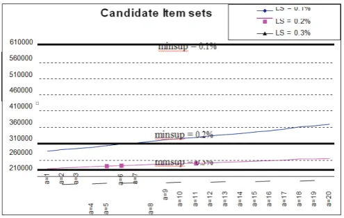
algorithms with only one minsup.) For our experiment, we use three very low LS values, 0.1%, 0.2%, and 0.3%. Figure 1 shows
the number of large itemsets found. The three thick lines give the numbers of large itemsets found using the existing approach of a
single minsup at 0.1%, 0.2% and 0.3% respectively. To show how
affects the number of large itemsets found by our method, we let = 1/and vary from 1 to 20. Figure 2 gives the corresponding numbers
of candidate itemsets in the experiment. Again the three thick lines give the number of candidate itemsets using the existing approach
of a single minsup at 0.1%, 0.2% and 0.3% respectively.
Fig. 1: Number of Large Itemsets Found
Fig. 2: Number of Candidate Itemsets
We see from Figure 1 that the number of large itemsets is significantly reduced by our method when is not too large. When
becomes larger, the number of large itemsets found by our method gets closer to that found by the single minsup method. The reason
is because when becomes larger more and more items’ MIS values reach LS. From our experiences, the user is usually satisfied with the large itemsets found at = 4. At = 4 and LS = 0.2%, for example, the number of large itemsets found by our method is less than 61% of that found by the single minsup method. From Figure 2, we
see that the corresponding numbers of candidate itemsets are also
much less. The execution times are roughly the same (hence are not shown here) because database scan dominates the computation
in this experiment. Below, we will see that for our real-life data set, the reductions in both the number of large itemsets found and the number of candidate itemsets used are much more remarkable because the item frequencies in our real-life data set vary a great deal. The execution times also drop drastically because the data set is small and the computation time is dominated by the itemsets generation.
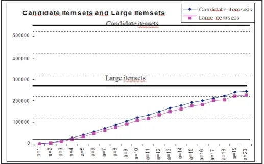
B. Application to real-life data
We tested the algorithm using a number of real-life data sets.
Due to confidentiality agreement, we are unable to provide the
details of the application. Here, we only give the characteristics
of the data. The data set has 55 items and 700 transactions. Each transaction has 14-16 items. Some items can appear in 500 transactions, while some may only appear in 30 transactions. The standard deviation of item frequencies in the data is 25.4% (the mean is 24.3%).
For this application, the user sets LS = 1%. The results are shown in Figure 3, which include both the numbers of candidate itemsets
and large itemsets found. The two thick lines show the number of candidate itemsets and the number of large itemsets found
respectively by the single minsup (= 1%) method. Our new method
reduces the numbers dramatically. For this application, the user is
happy with the large itemsets found at = 4. The number of large itemsets found by our method at = 4 is only 8.5% of that found
by the existing single minsup method. The drop in the number of candidate itemsets is even more drastic.
Fig. 3: Numbers of candidate itemsets and large itemsets
Fig. 4: Comparison of Execution Times in Percentage
Fig. 4 shows the execution time comparison in percentage. The execution time used by the single minsup method is set to 100%. We
can see that the proposed method also reduces the execution time
significantly (since this data set is small, the itemsets generation dominates the whole computation).
Note that for applications, the user can also assign MIS values
manually rather than using the formulas in Section IV.A.
V. Related Work
Association rule mining has been studied extensively in the past
[e.g., 2, 3, 5, 11, 4, 14, 10, 12, 1]. However, the model used in all these works is the same, i.e., with only one user-specified minimum support threshold [2].
Multiple-level association rule mining in [5] can use different
minimum supports at different levels of hierarchy. However, at the same level it uses only one minsup. For example, we have the taxonomy: milk and cheese are Dairy_product; and pork and beef
are Meat. At the level of Dairy_product and Meat, association rules
can have one minsup, and at the level of milk, cheese, pork and beef, there can be a different minsup. This model is essentially
the same as the original model in [2] because each level has its own association rules involving items of that level. Our proposed model is more flexible as we can assign a MIS value for each item. [13] presents a generalized multiple-level association rule
mining technique, where an association rule can involve items at any level of the hierarchy. However, the model still uses only one minsup.
It is easy to see that our algorithm MSapriori is a generalization of the Apriori algorithm [3] for single minsup mining. That is, when all MIS values are the same as LS, it reduces to the Apriori algorithm. A key idea of our algorithm MSapriori is the sorting of items in I according to their MIS use level-wise search, each
step of our algorithm is different from that of algorithm Apriori, from initialization, candidate itemsets generation to pruning of candidate itemsets.
This paper argues that a single minsup is insufficient for association rule mining since it cannot reflect the natures and frequency
differences of the items in the database. In real-life applications, such differences can be very large. It is neither satisfactory to set the minsup too high, nor is it satisfactory to set it too low. This paper
proposes a more flexible and powerful model. It allows the user
to specify multiple minimum item supports. This model enables us to found rare item rules yet without producing a huge number of meaningless rules with frequent items. The effectiveness of the new model is shown experimentally and practically.
References
[1] Aggarwal, C., and Yu, P. “Online generation of association
rules.” ICDE-98, 1998, pp. 402-411.
[2] Agrawal, R., Imielinski, T., Swami, A. “Mining association
rules between sets of items in large databases.” SIGMOD-
1993, 1993, pp. 207-216.
[3] Agrawal, R. and Srikant, R. “Fast algorithms for mining
association rules.” VLDB-94, 1994.
[4] Brin, S. Motwani, R. Ullman, J. and Tsur, S. “Dynamic
Itemset counting and implication rules for market basket data.” SIGMOD-97, 1997, pp. 255-264.
[5] Han, J. and Fu, Y. “Discovery of multiple-level association
rules from large databases.” VLDB-95.
[6] Lee, W., Stolfo, S. J., and Mok, K. W. “Mining audit data
to build intrusion detection models.” KDD-98.
[7] Liu, B., Hsu, W. and Ma, Y. Mining association rules with
multiple minimum supports. SoC technical report, 1999. [8] Liu, B., Hsu, W. and Ma, Y. “Pruning and Summarizing the
Discovered Associations” KDD-99, 1999.
[9] Mannila, H. “Database methods for data mining.” KDD-98
tutorial, 1998.
[10] Ng. R. T. Lakshmanan, L. Han, J. “Exploratory mining
and pruning optimizations of constrained association rules.”
SIGMOD-98, 1998.
[11] Park, J. S. Chen, M. S. and Yu, P. S. “An effective hash
based algorithm for mining association rules.” SIGMOD-95,
[12] Rastogi, R. and Shim, K. “Mining optimized association
rules with categorical and numeric attributes.” ICDE –98.
[13] Srikant, R. and Agrawal, R. “Mining generalized association
rules.” VLDB-1995, 1995.
[14] Srikant, R., Vu, Q. and Agrawal, R. “Mining association