Sensitivity Analysis of Six-Sigma Applied to a
Reliability Project
Salman T. Al-Mishari, S. M. A. Suliman
Abstract- The Six-Sigma DMAIC process was applied to improve the reliability on a group of water disposal pumps at a number of oil facilities. The anticipated cost avoidance in terms of production losses and maintenance costs was simulated to be about half the current costs. After the completion of the project, a number of what-if scenarios were conducted to assess the importance of each step in the DMAIC process. Examples of such scenarios are “what if the problem was not well Defined, Measured, Analyzed, Improved, or Controlled?” This paper presents the results of the simulated scenarios in terms of monetary figures. The purpose is to illustrate the significance of each step in the DMAIC process.
Index Term-- Risk centered maintenance, Six-Sigma, Sensitivity analysis, Machinery reliability.
I. INTRODUCTION
A number of approaches are available to design a periodic maintenance (PM) program. Some are very subjective such as Reliability Centered Maintenance and some are based on statistics and mathematical modeling. The Six-Sigma DMAIC process has been proposed as a tool to integrate the different approaches together [1]. Table I is a summary of the DMAIC process. This process was applied to a group of water disposal pumps at an existing
oil production facility. When the oil comes out of the ground, it is not pure oil but rather a mixture of oil, water, and gas. Separation is thus needed before further processing. To do the separation, Oil is taken to Gas Oil Separation Plants (GOSPs) at which the mixture goes in big traps where gas is taken from the top and sent to gas plants, oil is sent to refineries, and water is injected back to the ground by water injection pumps. In the past, the percentage of water in the mixture (called the water cut), was very low and not many injection pumps were needed. Despite that, enough redundancy of pumps was also installed to avoid production losses. Since the water is continuously injected back to the ground, the water cut has increased with time to a degree where the original redundancy is barely sufficient, and therefore, maximum availability is required to avoid expensive production losses. The DMAIC process was used to assist in developing an optimal design of a periodic maintenance (PM) program at the component level of these pumps. After the completion of the project, a question was raised of whether every element in the DMAIC process was indeed needed. The purpose of this paper is to examine the significance of each element and ultimately answer the raised question.
2
0 F 24
4 μ4, λ4
μ2, λ2 μ4, λ4
μ2, λ2
λS2
λS24
λS0
λS4
1
F 5
3 λS3
λS1 μ1, λ1
μ3, λ3
λS5 μ5, λ5
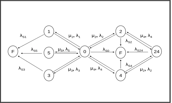
(1) solenoid, (2) discharge valve (3) relief valve (dumping ZV), (4) accumulator (5)thrust
Fig. 1. Markov model of the motivating problem
For the improve phase, a nonlinear programming model (Figure-1) was built and solved to find the optimal PM frequency for each component. For the control phase, a
TABLE I
SUMMARY OF DMAIC PROCESS
Phase Phase Elements Remarks
Define
Significance of Project The selected project has to be significant as verified by Organization’s accountant. The potential savings should at least be $250,000.
Scoping The project shall be scoped down to a limited manageable and yet significant size.
Process capability A base-line performance analysis shall be made at the beginning of analysis to gauge recommended improvement when implemented at later stage.
Measure
Adequacy of Measurement System.
The data used shall be verified to be correct before hand; e.g., counting every work order as a failure is an obvious flaw.
Measuring the factors
All potential factors that could cause the reliability problem should be measured. Measure tools are abundant in the Six-Sigma toolbox. Examples are process mapping, fishbone diagram, failure mode and effect analysis (FMEA).
Analyze Assessment of dominant
factors
Potential factors are then examined from which the dominant ones are assessed. Statistical analysis and techniques such as sampling, statistical comparison, correlation, and regression are highly promoted whenever applicable.
Improve Providing workability of the proposed solutions
Measuring before and after improvements.
Demonstration of solution effectiveness through design of experiment (DOE).
Demonstration of solution effectiveness by Simulation.
Control Adequate monitoring and
control
Improvement shall be sustained through close performance monitoring to detect process shifts and drifts early before they become expensive to correct.
II. RELATED LITERATURE
Maintenance strategies have evolved from reactive to proactive through the implementation of some type of periodic maintenance (PM). There are a number of approaches for selecting PM activities and setting their intervals. Some of these approaches are subjective such as reliability centered maintenance (RCM) and total productive maintenance (TPM); and others are more objective such as statistical based models. Reliability Centered Maintenance (RCM) is usually based on subjective estimation of risk by a group of subject matter experts via risk models and charts such as Failure Mode Effect Analysis (FMEA) charts [2]. The classical version of RCM is criticized of being very rigorous and resource intensive since every potential failure mode is analyzed [3]. Streamlined versions were, therefore, proposed to limit the scope to the dominant functions and failure modes, or to replicate results to other similar applications[4], and [5]. Despite the hot discussion by peer RCM practitioners between supporters and criticizers of streamlined methods, such methods were reported to achieve significant savings [6]. Examples of RCM applications include a wide range of plant equipment such
as gas compression systems, boilers, and turbine auxiliaries [4], [7], and [8].
TPM is a major departure from the “you operate, I maintain” philosophy and rather encourages total employee involvement. TPM recognizes that equipment operators are continually in contact with their machines, which allows them to detect small changes in the performance or behavior of the equipment. Operators can proactively address many of these small issues themselves and can provide early warning for problems that require specialized skills to correct [10], and [11]. TPM, however, focuses more on who should do the PM more than what PM activities should be done. There is, thus, still a need for other approaches to identify the needed activities. Both RCM and TPM are subjective in nature. They depend heavily on subject matter expertise to come up with a list of PM tasks and to decide who can best carry them out.
methodologies for handling partial failures. Honkanen [11] suggests that the main reason seems to be that it is very difficult to model system degradation in terms of partial failures of a component or a combination of components. Although it’s rare, some work is available in the literature that addresses degradation and the effect of maintenance on reliability. The basis of these models is the realization that frequent maintenance comes at cost while infrequent maintenance leads to costly consequences. The objective, therefore, is to balance these two costs. Examples of these models are Profit/cost optimization models [12] - [14], Markov state models [15] and [16], and Petri Nets [17].
In practice, the choice between subjective and objective models is sometimes very difficult. Each has its own merits and limitations. In an attempt to capture the merits of both types and contain the limitations, Six-Sigma has been proposed as an integration tool. Six-Sigma has proven very successful in the manufacturing, service, and transactional applications and also seems to be very promising for reliability applications. Six-Sigma has been successfully applied to the motivating application [1]. It was questioned, however, if every element of the Six-Sigma DMAIC process was indeed needed.
III. ASSESSING THE NEED FOR EACH DMAIC
ELEMENT
The motivating application is used to assess the need for each DMAIC element. The assessment is organized in the same order presented in Table II.
A. Define Phase
Project Significance
The motivating project was competing with another reliability equipment project. The competing project was addressing a mechanical seal reliability concern raised at another facility. This project was triggered when a newly-assigned facility manager noticed that during three consecutive morning reports, a new seal maintenance activity was reported every morning. He suggested that the reliability of mechanical seals should perhaps be improved. Becoming a manager’s concern, it received attention by a number of plant personnel and a number of improvement ideas were, thus, voluntarily proposed for consideration. Without analyzing the project significance, this competing project would’ve had a priority and would, therefore, be selected instead of the subject mechanical seal project.
The what-if question would, then, be whether this was the right selection given that there are resources to conduct only one project. To answer this question, recent
maintenance history was carefully examined which revealed that most of the maintenance done on the competing equipment was minor with a total cost of about $25,000 dollars over a period of 27 months; i.e., an average annual cost of $11,000.
TABLE II
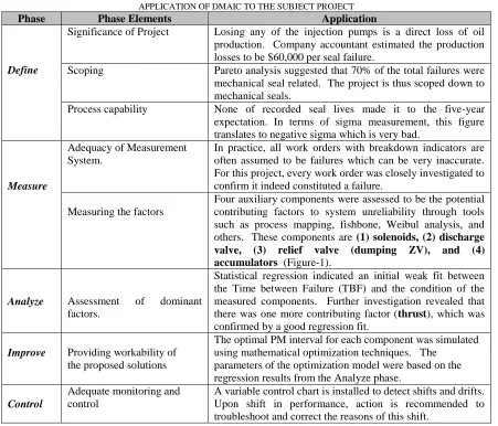
APPLICATION OF DMAIC TO THE SUBJECT PROJECT
Phase Phase Elements Application
Define
Significance of Project Losing any of the injection pumps is a direct loss of oil production. Company accountant estimated the production losses to be $60,000 per seal failure.
Scoping Pareto analysis suggested that 70% of the total failures were mechanical seal related. The project is thus scoped down to mechanical seals.
Process capability None of recorded seal lives made it to the five-year expectation. In terms of sigma measurement, this figure translates to negative sigma which is very bad.
Measure
Adequacy of Measurement System.
In practice, all work orders with breakdown indicators are often assumed to be failures which can be very inaccurate. For this project, every work order was closely investigated to confirm it indeed constituted a failure.
Measuring the factors
Four auxiliary components were assessed to be the potential contributing factors to system unreliability through tools such as process mapping, fishbone, Weibul analysis, and others. These components are (1) solenoids, (2) discharge valve, (3) relief valve (dumping ZV), and (4) accumulators (Figure-1).
Analyze Assessment of dominant
factors.
Statistical regression indicated an initial weak fit between the Time between Failure (TBF) and the condition of the measured components. Further investigation revealed that there was one more contributing factor (thrust), which was confirmed by a good regression fit.
Improve Providing workability of the proposed solutions
The optimal PM interval for each component was simulated using mathematical optimization techniques. The
parameters of the optimization model were based on the regression results from the Analyze phase.
Control
Adequate monitoring and control
A variable control chart is installed to detect shifts and drifts. Upon shift in performance, action is recommended to troubleshoot and correct the reasons of this shift.
Scoping
Pareto analysis suggested that mechanical seals were the number-one contributors to the unreliability of the subject pumps followed by the bearings. Mechanical seals contributed to 70% of the total unreliability and bearings contributed to 20%. The project was thus scoped down to mechanical seals. Without this scoping analysis, it was likely to invest the investigation resources on bearings instead of mechanical seals. The result would have been a loss of opportunity. To quantify this potential loss of saving opportunity, maintenance history over a four-year period was examined which showed that the cost of unreliability due to bearings was only $450,000 while the cost of unreliability due to seals is $3,000,000. If we assume that it would have been possible to make 50% savings on bearings just as we did with on seals. This would mean savings of $225,000 (50% x $450,000) instead of $1,500,000 (50% x $3,000,000); i.e., an annual
loss of saving opportunity of $1,250,000 ($1,500,000 - $225,000).
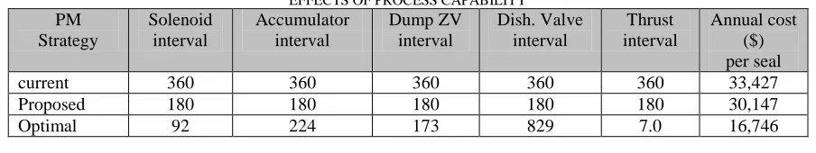
Process Capability
the three different scenarios; current PM intervals of 360 days, the proposed PM intervals of 180 days, and the optimal intervals. This would mean savings of $3,280 ($33,427 - $30,147) instead of $16,681 ($33,427 –
16,746); i.e., an annual loss of saving opportunity of $13,401 ($16,681 – 3,280).
TABLE III
EFFECTS OF PROCESS CAPABILITY
PM Strategy
Solenoid interval
Accumulator interval
Dump ZV interval
Dish. Valve interval
Thrust interval
Annual cost ($) per seal
current 360 360 360 360 360 33,427
Proposed 180 180 180 180 180 30,147
Optimal 92 224 173 829 7.0 16,746
B. Measure Phase
Adequacy of Measurement System
Every work order in this project was carefully examined to ensure that it indeed represented a mechanical seal failure and all related data was correct. If this step was not carefully conducted, the result would’ve been a poor regression model. Consequently, it would have been merely relied on subject matter experts (SMEs) to estimate the Markov model parameters. Based on a preliminary survey and initial judgment of SMEs, it was believed that four system subcomponents were the major contributors to the existing level of unreliability. The MTBF on these components was subjectively estimated to be about three years; which corresponds to a failure rate of 0.0009 per day. Upon failure of any of these components, it was judged that the system MTBF will deteriorate from 5 years to one year (i.e., from 0.00056 to 0.00278 per day).
Based on parameters estimated above, the transition matrix would change. Also, there would be no fifth component (Thrust) since this component was only identified after the initial regression analysis. The SMEs also indicated that they would consider the possibility of interaction effects is remote, and therefore, they would not consider it.
Solving the NLP model of [1] based on the above estimated parameters gives incorrect optimal PM intervals (Table IV). These incorrect optimal PM intervals, as simulated using the correct NLP model, do not generate any cost savings. In the contrary, they add extra cost as compared to the current PM program; e.g., $ 37,580 vs. $33,430.
TABLE IV
EFFECTS OF ADEQUACY OF MEASUREMENT SYSTEM
PM Strategy
Solenoid interval
Accumulator interval
Dump ZV interval
Dish. Valve interval
Thrust interval
Annual Cost ($) per seal
Current 360 360 360 360 360 33,427
Incorrect Optimal
43 62.4 77.9 91.5 360 37,580
Optimal 92 224 173 829 7.0 16,746
Measuring the Factors
A number of factors (arising as system subcomponents) have been identified to contribute to the subject unreliability problem. The question is what would happen if there was a failure to identify any of these factors? The direct answer to this question would be the result of a poor regression model which will lead to relying on subjective judgment as an alternative. If we assume, however, that the effects associated with any factor (as long as it is
TABLE V
EFFECTS OF MEASURING THE FACTORS
PM Strategy
Solenoid Interval
(N)
Accumulator Interval
(A)
Dump ZV Interval (Z)
Dish. Valve Interval
(D)
Thrust Interval
(T)
Annual Cost per seal
Current 360 360 360 360 360 33,427
Removal of N 100,000 224 173 829 7.0 19,120
Removal of A 92 100,000 173 829 7.0 18,659
Removal of Z 92 224 100,000 829 7.0 20,003
Removal of D 92 224 173 100,000 7.0 17,136
Removal of T 92 224 173 829 100,000 40,036
Optimal 92 224 173 829 7.0 16,746
The potential opportunity loss varies depending on which factor is removed. In this example, it varies between $390 (the difference between the optimal and the removal of D) to $23,290 (the difference between the optimal and the removal of T). It’s, thus, concluded that careful measurement of the contributing factors is a critical DMAIC element for the improvement process.
C. Analyze Phase
Heuristic Assignment of Model Parameters
The objective of the Analyze phase is to identify the dominant factors and establish their relationship to the problem using scientific tools such as statistics whenever possible. In this project, statistical regression was the tool used to establish this relationship. An alternative venue would have been to establish this relationship heuristically; i.e., based on mere subjective judgment. The question is what would have happened if that was the case? Model parameters would have been merely based on SMEs. The loss of opportunity is thus the same as that of Table V.
D. Improve Phase
Demonstrating the Effectiveness of Solutions
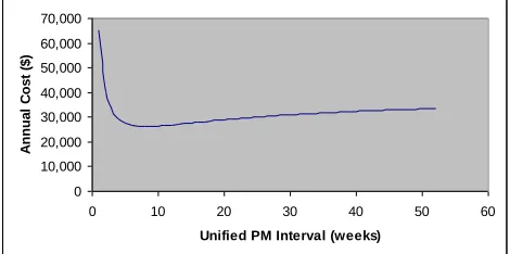
A mathematical optimization model was built to search for the optimal solution. The model building went through a number of hurdles to a point where it was suggested to take different approaches. One proposed approach was to unify the PM intervals for all components which will make the search for the optimal solution easier. The question is what would have happened if this approach was taken for setting the PM intervals instead of the NLP model? Figure 2 illustrates the results of this exercise. The optimal unified PM interval as shown in the figure is 8 weeks
corresponding to an annual cost of $26,288. A more fine-tuned search (by days) suggests a unified PM interval of 57 days corresponding to an annual cost of $26,285. This dollar figure when compared to the real optimal cost of $16,681 corresponds to a potential loss of saving opportunity of around $9,604 ($26,285-$16,681) per seal.
0 10,000 20,000 30,000 40,000 50,000 60,000 70,000
0 10 20 30 40 50 60
Unified PM Interval (weeks)
A
nnu
a
l
C
os
t
($
)
Fig. 2. Effects of verifying improvements
E. Control Phase
Inadequate Monitoring and Control
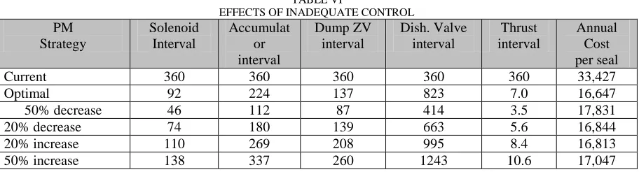
To study the effect of improper control, a number of scenarios are studied regarding what would happen if the PM intervals are properly controlled? i.e., allowing them to shift and drift. Four scenarios are studied as shown in Table VI. These scenarios correspond to allowing the PM intervals to shift:
TABLE VI
EFFECTS OF INADEQUATE CONTROL
PM Strategy
Solenoid Interval
Accumulat or interval
Dump ZV interval
Dish. Valve interval
Thrust interval
Annual Cost per seal
Current 360 360 360 360 360 33,427
Optimal 92 224 137 823 7.0 16,647
50% decrease 46 112 87 414 3.5 17,831
20% decrease 74 180 139 663 5.6 16,844
20% increase 110 269 208 995 8.4 16,813
50% increase 138 337 260 1243 10.6 17,047
As seen in Table VI, the potential opportunity loss due to inadequate control can be as much as $1184 ($17,831 - $16,647) for a 50% decrease on PM intervals. This loss corresponds only to one mechanical seal setup. For all the 90 setups included in the project, this adds up to a significant amount of potential loss (about $106,560 per year).
IV. SUMMARY AND CONCLUDING REMARKS The potential losses due to missing any element of the DMAIC process are very significant. In industrial practice, there is a tendency toward quick solutions, judgment, and a great deal of assumptions. Many improvement projects are not carefully selected. Assessment of contributing factors is often based on very subjective judgment. Recommendations are sometimes proposed without very careful analysis and often not verified for credibility. Shifts and drifts often occur. All these factors have a very significant impact that can sometimes be very much hidden simply
because
it’s often not measured. The work reported in this paper attempts to illustrate the potential losses of missing these important elements through a real example.REFERENCES
[1] S. Al-Mishari, and S. M. A. Suliman, “Modelling preventive maintenance for auxiliary components,” Journal of Quality in Maintenance Engineering, vol. 14, no. 1, pp 59-70, 2008. [2] D. H. Stamatis, “Failure mode and effect analysis: FMEA
from theory to execution,” in ASQ quality Press, Milwaukee, Wisconsin 1995.
[3] SAE JA1011, “Evaluation criteria for reliability-centered maintenance (RCM) processes”, International Society of Automotive Engineers, 1999.
[4] B. S. Hauge, “Reliability centered maintenance and risk assessment,” IEEE proceedings Annual reliability and maintainability symposium, pp 36-40, 2001.
[5] S. Turner, (2005). P M Optimisation: maintenance analysis of the future, PMOptimisation website at www.pmoptimisation.com
[6] J. Moubray, “Reliability centered maintenance,” 2nd ed.
New York, NY, USA: Industrial Press Inc., 1997.
[7] F. Backlund, and P. A. Akersten, “RCM introduction: process and requirements management aspects,” Journal of Quality in Maintenance Engineering, vol. 9, no. 3, pp 251-264, 2003.
[8] S. Srikrishna, G. S. Yadava, and P.N. Rao, “Reliability-centered maintenance applied to power plant auxiliaries”, Journal of Quality in Maintenance and Engineering, vol. 2, no. 1, pp. 3-14, 1996.
[9] S. Nakajima, “Introduction to TPM,” Productivity Press, Cambridge, Massachusetts, 1988.
[10] J. G. Noguera, (2006), "Six-sigma course notes," J.G. Noguera & Associates, http://www.jgna.com/
[11] T. Honkanen, “Modeling industrial maintenance systems and the effects of automatic condition monitoring,” PhD Dissertation, Helsinki University of technology, 2004. [12] R. L. Kenyon, and R. J. Newell, “Steady-state availability of
k-out-of-n: G system with single repair,” IEEE Transactions on Reliability, vol. 32, pp. 188-190, 1983.
[13] R. V. Canfield, “Cost optimization of periodic preventive maintenance”, IEEE Tran. Reliability, vol. 35, pp. 78-81, 1986.
[14] L. M. Millart, and S. M. Pollock, “Cost-optimal condition-monitoring for predictive maintenance of 2-phase systems,” IEEE Transactions on Reliability, vol. 51, pp. 71-75, 2002. [15] J. Endrenyi, G. J. Anders, and A. M. Silva, “Probability
evaluation of the effect of maintenance on reliability - an application,” IEEE Transactions on Power Systems, vol. 13, pp 576-583. 1998.
[16] D. Chen, and K. S. Trivedi, “Optimization for condition-based maintenance with semi-Markov decision process,” Reliability Engineering and System Safety, vol. 90, pp. 25– 29, 2005.
[17] M. Hosseini, R. M. Kerr, and R. B. Randall, “An inspection model with minimal and major repair,” IEEE Transactions on Reliability, vol. 49, pp. 88-98, 2000.
Salman T. Al-Mishari is with Machinery Reliability Unit, Saudi Aramco, Dahran, KSA ([email protected]).