e-ISSN: 2278-067X, p-ISSN: 2278-800X, www.ijerd.com
Volume 10, Issue 6 (June 2014), PP.42-51
Bifurcation Analysis of Prey-Predator Model with
Harvested Predator
Vijaya Lakshmi. G.M
1, Gunasekaran. M
2,*, Vijaya. S
31Department of Mathematics, Indira Institute of Engineering and Technology,Thiruvallur-631 203. 2PG Department of Mathematics, Sri Subramaniya Swamy Government Arts College, Tiruttani-631 209.
3
PG& Research Department of Mathematics, Annamalai university, Chidambaram-608 002.
Abstract:- This paper aims to study the effect of harvested predator species on a Holling type IV Prey-Predator model involving intra-specific competition. Prey-predator model has received much attention during the last few decades due to its wide range of applications. There are many kind of prey-predator models in mathematical ecology. The Prey-predator models governed by differential equations are more appropriate than the difference equations to describe the prey-predator relations. Harvesting has a strong impact on the dynamic evolution of a population. This model represents mathematically by non-linear differential equations. The locally asymptotic stability conditions of all possible equilibrium points were obtained. The stability/instability of non-negative equilibrium and associated bifurcation were investigated by analysing the characteristic equations. Moreover, bifurcation diagrams were obtained for different values of parameters of proposed model.
Keywords:- Prey-Predator model, Holling type functional response, Harvesting, Bifurcation.
I.
INTRODUCTION
The prey-predator model with differential equations give rise to more efficient computational models for numerical simulations and it exhibits more plentiful dynamical behaviours than a prey-predator model with difference equations of the same type. There has been growing interest in the study of Prey-Predator models described by differential equations. In ecology, predator-prey or plant herbivore models can be formulated as differential equations. It is well known that one of the dominant themes in both ecology and mathematical ecology is the dynamic relationship between predators and their prey. One of the important factors which affect the dynamical properties of biological and mathematical models is the functional response. The formulation of a predator-prey model critically depends on the form of the functional response that describes the amount of prey consumed per predator per unit of time, as well as the growth function of prey [1,15]. That is a functional response of the predator to the prey density in population dynamics refers to the change in the density of prey attached per unit time per predator as the prey density changes.
In recent years, one of the important Predator – Prey models with the functional response is the Holling type – IV, originally due to Holling which has been extensively studies in many articles [4-6, 11]. Two species models like Holling type II, III and IV of predator to its prey have been extensively discussed in the literature [2-6,9,16]. Leslie-Gower predator- prey model with variable delays, bifurcation analysis with time delay, global stability in a delayed diffusive system has been studied [8,12,14]. Three tropic level food chain system with Holling type IV functional responses , the discrete Nicholson Bailey model with Holling type II functional response and global dynamical behavior of prey-predator system has been revisited [7,10,11,13].The purpose of this paper is to study the effect of harvested predator species on a Holling type IV prey predator model involving intra-specific competition. We prove that the model has bifurcation that is associated with intrinsic growth rate. The stability analysis that we carried out analytically has also been proved.
In this paper we consider the following Lotka-Volterra Prey- Predator system:
( )
( )
(1)
( )
dx
xq x
yp x
dt
dy
yp x
y
dt
here
x
(0), (0)
y
0,
Where
x and y
represent the prey and predator density, respectively.
p x
( ) and ( )
q x
are so-called predator and prey functional response respectively.
,
0
are the conversion and predator`s death rates,respectively. If
p x
( )
mx
a
x
refers to as Michaelis-Menten function or a Holling type – II function, where0
m
denotes the maximal growth rate of the species anda
0
is half-saturation constant. Another class of response functions are Holling type-III and Holling type-IV function, in which Holling type – III function is2 2
( )
mx
p x
a
x
and Holling type-IV function is( )
2mx
p x
a
x
. The Holling type – IV function otherwiseknown as Monod-Haldane function which is used in our model. The simplified Monod-Haldane or Holling type – IV function is a modification of the Holling type-III function. In this paper, we focus on effect of harvested predator species on a Holling type IV prey-predator model involving intra-specific competition and establish results for boundedness, existence of a positively invariant and the locally asymptotical stability of coexisting interior equilibrium.
II.
THE MODEL
The prey-predator systems have been discussed widely in the many decades. In the literature many studies considered the prey-predator with functional responses. However, considerable evidence that some prey or predator species have functional response, because of the environmental factors. It is more appropriate to add the functional responses to these models in such circumstances. For example a system is suggested in (1), where
x t
( )
andy t
( )
represent densities or biomasses of the prey-species and predator species, respectively;( )
p x
andq x
( )
are the intrinsic growth rates of the predator and prey respectively;
and
are the death rates of prey and predator respectively.If
( )
21
mx
p x
x
andq x
( )
ax
1
x
, inp x
( )
assuminga
1
in general function, wherea
is thehalf-saturation constant in the Holling type IV functional response, then Eq.(1) becomes
22
1
1
(2)
1
my
x
x a
x
x
mx
y
y
x
Here
a
, ,
and m
are all positive parameters.
Now introducing harvesting factor on predator with intra-specific competitions, the Eq. (2) becomes
2
0 2
1
(3)
1
my
x
x a bx
x
e mx
y
y
y
q E
x
With
x
(0), (0)
y
0
and
, , , , , ,
m a b e
,q
0and E
are all positive constants.
attack rate of prey by the predator ,
e
represents the conversion rate,E
is harvesting effort and finallyq
0 is the catchability coefficient. The catch-rate functionq E
0 is based on the catch-per-unit-effort (CPUE).III.
EXISTENCE AND LOCAL STABILITY ANALYSIS WITH PERSISTENCE
In this section, we first determine the existence of the fixed points of the differential equations (3), and then we investigate their stability by calculating the Eigen values for the variation matrix of (3) at each fixed point. To determine the fixed points, the equilibrium is the solution of the pair of equations below:
2
0 2
0
1
(4)
0
1
my
x a bx
x
e mx
y
y q E
x
By simple computation of the above algebraic system, it was found that there are three nonnegative fixed points:
(i)
E
0
0, 0
is the trivial equilibrium point always exists.(ii)
E
1a
, 0
b
is the axial fixed point always exists, as the prey population grows to the carrying capacity in the absence of predation.(iii)
E
2
x y
*,
*
is the positive equilibrium point exists in the interior of the first quadrant if and only if there is a positive solution to the following algebraic nonlinear equationsWe have the following polynomial with fifth and third degree.
* 5 4 3 2
5 4 3 2 1 0
* 3 2
3 2 1 0
x
A x
A x
A x
A x
A x
A
y
B x
B x
B x
B
(5)Where
5 2 2 4 2 2 3 2 2
2
,
,
,
b
a
b
A
A
A
e
m
e
m
e
m
0 0
2 2 2 1 2 2 0 2 2
2
,
,
q E
a
m
mq E
a
b
A
A
A
e
m
e m
e
m
e
m
and
3
,
2,
1,
0b
a
b
a
B
B
B
B
m
m
m
m
Remark 1: There is no equilibrium point on
y
axis as the predator population dies in the absence of its prey.Lemma: For values of all parameters, Eqn.(3) has fixed points, the boundary fixed point and the positive fixed point
x y
*,
*
, wherex y
*,
* satisfy2
0 2
1
(6)
1
my
a bx
x
e mx
y
q E
x
Now we study the stability of these fixed points. Note that the local stability of a fixed point
x y
,
is determined by the modules of Eigen values of the characteristic equation at the fixed point.The Jacobian matrix J of the map (3) evaluated at any point
x y
,
is given by11 12 21 12
( , )
a
a
(7)
J x y
a
a
Where
2
11 2 2
1
2
1
my
x
a
a
bx
x
; 12 21
mx
a
x
2
21 2 2
1
1
e my
x
a
x
; 22 22
01
e mx
a
y
q E
x
and the characteristic equation of the Jacobian matrix
J x y
,
can be written as
2
,
,
0
p x y
q x y
,Where
,
11 22
p x y
a
a
,q x y
,
a a
11 22
a a
12 21.In order to discuss the stability of the fixed points, we also need the following lemma, which can be easily proved by the relations between roots and coefficients of a quadratic equation.
Theorem: Let
F
( )
2
P
Q
. Suppose thatF
1
0
,
1,
2 are two roots ofF
( )
0
. Then (i)1
|
| 1
and|
2| 1
if and only ifF
1
0
andQ
1
;(ii)
|
1| 1
and|
2| 1
(or|
1| 1
and|
2| 1
) if and only ifF
1
0
; (iii)|
1| 1
and|
2| 1
if and only ifF
1
0
andQ
1
;(iv)
1
1
and|
2| 1
if and only ifF
1
0
andP
0, 2
;(v)
1 and
2are complex and|
1| 1
and|
2| 1
if and only ifP
2
4
Q
0
andQ
1
.Let
1 and
2 be two roots of (7), which are called Eigen values of the fixed point
x y
,
. We recall some definitions of topological types for a fixed point
x y
,
. A fixed point
x y
,
is called a sink if|
1| 1
and|
2| 1
, so the sink is locally asymptotic stable.
x y
,
is called a source if|
1| 1
and|
2| 1
, so the source is locally un stable.
x y
,
is called a saddle if|
1| 1
and|
2| 1
(or|
1| 1
and|
2| 1
). And
x y
,
is called non-hyperbolic if either|
1| 1
and|
2| 1
.Proposition 1: The Eigen values of the trivial fixed point
E
0
0, 0
is locally asymptotically stable if
0
1
1,
a
E
q
(i.e.,)E
0 is sink point, otherwise unstable if
0
1
1,
a
E
q
and alsoE
0 issaddle point if
0
1
1,
a
E
q
,E
0 is non-hyperbolic point if
0
1
1,
a
E
q
.0 0
0
(0,0)
0
a
J
q E
Hence the Eigen values of the matrix are
1= ,
a
2=
q E
0Thus it is clear that by Theorem,
E
0 is sink point if|
1,2| 1
0
1
1,
a
E
q
,that isE
0 is locallyasymptotically stable.
E
0 is unstable (i.e.,) source if|
1,2| 1
0
1
1,
a
E
q
.And also
E
0 is saddle point if|
1| 1, |
2| 1
0
1
1,
a
E
q
,E
0 is non-hyperbolic pointif
|
1| 1 or |
2| 1
0
1
1,
a
E
q
.Proposition 2: The fixed point
E
1a
, 0
b
is locally asymptotically stable, that is sinkif
2 2
2 2 0
1
1 and
eab m
a
b
a
E
q a
b
;E
1 is locally unstable, that is sourceif
2 2
2 2 0
1
1 and
eab m
a
b
a
E
q a
b
;E
1 is a saddle point if
2 2 2 2 01
1 and
eab m
a
b
a
E
q a
b
andE
1 is non-hyperbolic point ifeither
2 2
2 2 0
1
1 or
eab m
a
b
a
E
q a
b
.Proof: One can easily see that the Jacobian matrix at
E
1 is2 2 1 0 2 2
, 0
0
ab m
a
a
a
b
J
eab m
b
Eq
a
b
Hence the Eigen values of the matrix are
|
1|= , |
a
2|=
eab m
2 2Eq
0a
b
By using Theorem, it is easy to see that,
E
1 is a sink if
2 2
2 2 0
1
1 and
eab m
a
b
a
E
q a
b
1
E
is a source if
2 2
2 2 0
1
1 and
eab m
a
b
a
E
q a
b
;E
1 is a saddleif
2 2
2 2 0
1
1 and
eab m
a
b
a
E
q a
b
; andE
1 is a non-hyperbolic if either
2 2 2 2 01
1 or
eab m
a
b
a
E
q a
b
.Remark 2: If
2
Tr J
(
2)
Det J
(
2)
0
, then the necessary and sufficient condition for linear stability areTr J
(
2)
0 and
Det J
(
2)
0
.IV.
LOCAL STABILITY AND DYNAMIC BEHAVIOUR AROUND
INTERIOR FIXED POINT
E
2Now we investigate the local stability and bifurcations of interior fixed point
E
2. The Jacobian matrix atE
2 is of the form
2 2 2 2 2 2 * * * 2 * * * * 2 * * * * 0 2 * *1
2
1
1
( ,
)
(8)
1
2
1
1
my
x
mx
a
bx
x
x
J x y
e my
x
e mx
y
q E
x
x
Its characteristic equation is
F
( )
2
Tr J
(
2)
Det J
(
2)
0
whereTr
is the trace andDet
is the determinant of the Jacobian matrixJ E
(
2)
defines in Eq.(8), (by Lemma) where
2 2 2 * * * *2 2 * 0 1 2
*
1
( ) 2 2 = +
1 1
my x e mx
Tr J a bx y Eq
x x
and
2 2 2 2 2* * 2 2 * * *
* *
2 2 * 0 3 1 2 3
* *
1 1
( ) 2 2 = .
1
1 1
my x e mx e m x y x
Det J a bx y q E
x x x
2 2 2 * * * *1 2 2 * 0
*
1
2 , 2
1 1
my x e mx
a bx y Eq
x x
and
2
2
2 2 * * *
3 3
*
1
1
e m x y x
x
2
E
is stable if
3 2
* *
* * * *
0 0
E > a 2 bx y ex yx ex y
q q
(9)
and
2
2 2 2 2
2 2 * * * *
*
2
* * * * * *
0 0
1 2
E <
1 1 2 1 1
e m x y x
y e mx
q
q x q x a bx x my x
(10)
If both equations (9) and (10) are satisfied, then the interior equilibrium point will be stable.
V.
NUMERICAL SIMULATION
The global dynamical behaviour of the non-linear model system (3) in the positive octant is investigated numerically. Under the bifurcation analysis of the model (3), very rich and complex behaviours are observed, presenting various sequences of period-doubling bifurcation leading to chaotic dynamics or sequences of period-halving bifurcation leading to limit cycles.
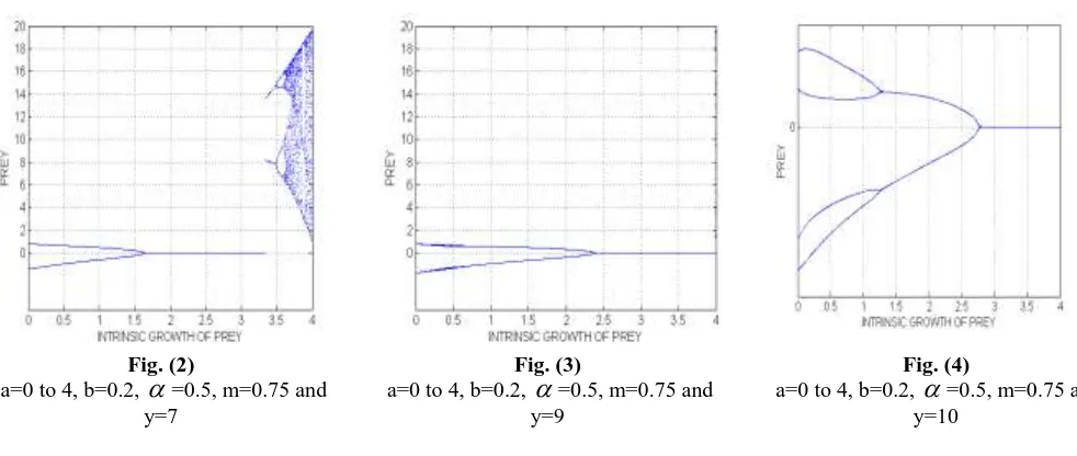
The prey-predator system (3) with the effect of harvested predator species on a Holling type IV functional response, intra-specific competition exhibits a variety of dynamical behaviour in respect of the population size. We first plotted the diagrams for the prey system with various intrinsic growth rates. The Fig.(1) shows that stabilized prey density first bifurcates 2 cycles, 4 cycles, forms a little chaos and then forms chaotic band with intrinsic prey growth rate 0 to 4 in the absence of the predator. That is, period-doubling bifurcation leading to chaotic dynamics. Next we introduce predator, then for various predator values.
Fig. (1)
a=0 to 4, b=0.2,
=0.5, m=0.75 in the absence of predatorFig. (2)
a=0 to 4, b=0.2,
=0.5, m=0.75 and y=7Fig. (3)
a=0 to 4, b=0.2,
=0.5, m=0.75 and y=9Fig. (4)
a=0 to 4, b=0.2,
=0.5, m=0.75 and y=10Fig.(5) shows prey growth rate which leads to period-halving bifurcation leading to limit cycles.
Fig. (5)
a=0 to 4, b=0.2,
=0.5, m=0.75and y = 13Fig. (6)
m=0 to 5, e=0.4,
=0.5,x
=0.5,y
=5,q
0=0.5 andE
=1.5Fig. (7)
m=0 to 5, e=0.4,
=0.5,x
=10,y
=5,q
0=0.5 andE
=1.5Fig. (8)
m=0 to 5, e=0.4,
=0.5,x
=1.5,y
=5,q
0=0.5 andE
=2Fig.(9) and Fig.(10) shows clearly the evidence of the route to chaos through the cascade of period-halving bifurcation respectively for the prey values
x
=1.5 andx
=6.Fig. (9)
m=0 to 5, e=0.4,
=0.5,x
=1.5,y
=5,q
0=0.5 andE
=3Fig. (10)
m=0 to 5, e=0.4,
=0.5,x
=6,y
=5,q
0=0.5 andE
=3 The above plots have been generated by using MATLAB 7 software.VI.
CONCLUSION
In this paper, we have investigated the complex behaviours of two species prey- predator system as a set of differential equations with the effect of harvested predator species on a Holling type IV functional response and intra-specific competition in the closed first quadrant, and showed that the unique positive fixed point of system (3) can undergo bifurcation and chaos. Bifurcation diagrams have shown that there exists much more interesting dynamical and complex behaviour for system (3) including periodic doubling cascade, periodic windows and chaos. All these results showed that for richer dynamical behaviour of the prey-predator differential equation model (3) under periodical perturbations compared to the difference equation model. The system is examined via the techniques of local stability analysis of the equilibrium points from which we obtain the bifurcation criterion.
rate among the predator species with harvesting effort and catchability coefficient. Thus it is observed that even a small variation in parameters
a
with zero predators andm
withe
andq
0 may cause a shift form limit cycles to chaos and vice-versa respectively. This study gives support to the view that two species prey-predator model with a system of differential equations are able to generate unpredictable and complex behaviour with small perturbations in parameters.REFERENCES
[1]. Agiza. H.N, Elabbasy. E.M, EK-Metwally,Elsadany. A.A, Chaotic dynamics of a discrete prey-predator model with Holling type II, Nonlinear analysis: Real world applications 10 (2009), pp.116-129.
[2]. Aziz-Alaoui. M.A and Daher Okiye. M, Boundedness and global stability for a predator-prey model with modified Leslie-gower and Holling-type II schemes, 16 (2003), pp.1069-1075.
[3]. Baba I. Camara and Moulay A. Aziz-Alaoui, Complexity in a prey predator model, International conference in honor of Claude Lobry , Vol.9 (2008), pp.109-122.
[4]. Hongying lu and Weiguo wang, Dynamics of a delayed discrete semi-ratio dependent predator-prey system with Holling type IV functional response, Advances in difference equations (2011), pp.3-19. [5]. Lei zhang, Weiming wang, Yakui xue and Zhen jin, Complex dynamics of a Holling-type IV
predator-prey model, (2008), pp.1-23.
[6]. Manju Agarwal, Rachana Pathak, Harvesting and hopf bifurcation in a prey-predator model with Holling type IV functional response, International journal of mathematics and soft computing, Vol.2, No.1 (2012), pp.83-92.
[7]. Moghadas. S.M, and Corbett. B.D, Limit cycles in a generalized Gause-type predator-prey model, Chaos, Solitons and Fractals 37 (2008), pp.1343-1355.
[8]. Shanshan chen, Junping shi and Junjie wei, Global stability and hopf bifurcation in a delayed diffusive Leslie-gower predator-prey system, International journal of bifurcation and chaos, Vol.22, No.3 (2012), pp.1-11.
[9]. Shanshan chen, Junping shi, Junjie wei, The effect of delay on a diffusive predator-prey system with Holling type-II predator functional response, Communications on pure and applied analysis, Vol.12, No.1 (2013), pp.481-501.
[10]. Shigui Ruan and Dongmei Xiao, Global analysis in a predator-prey system with nonmonotonic functional response, Society for industrial and applied mathematics, Vol.61, No.4 (2001), pp.1445-1472.
[11]. Shuwen zhang, Fengyan wang, Lansun chen, A food chain model with impulsive perturbations and Holling IV functional response, Chaos, Solitons and Fractals, 26 (2005), pp.855-866.
[12]. Tianwei zhang, Xiaorong gan, Existence and permanence of almost periodic solutions for Leslie-Gower predator-prey model with variable delays, Electronic journal of differential equations, No.105 (2013), pp.1-21.
[13]. Vijaya Lakshmi. G.M, Vijaya. S, Gunasekaran. M, Complex effects in dynamics of prey-predator model with Holling type II functional response, International journal of emerging science and engineering, Vol.2, Issue.3 (2014), pp.2319-6378.
[14]. Wen zhang, Haihong Liu, Chenglin xu, Bifurcation analysis for a Leslie-gower predator-prey system with time delay, International journal of nonlinear science, Vol.15, No.1 (2013), pp.35-44.
[15]. Yujing Gao, Dynamics of a ratio-dependent predator-prey system with a strong Allee effect, Discrete and continuous dynamical systems series B, Vol.18, No.9 (2013), pp.2283-2313.