Graphical Kernel System (GKS)
Ravi Sangwan, Pankaj Gupta
Dronacharya College of Engineering
Abstract: The Graphical Kernel System (GKS) was the first
ISO standard for low-level computer graphics, introduced in 1977. The Graphical Kernel System (GKS) is a document produced by the International Standards Organization (ISO) which defines a common interface to interactive computer graphics for application programs. GKS has been designed by a group of experts representing the national standards institutions of most major industrialized countries. This paper will tell you everything about GKS and all the primitives used in this system. GKS provides a set of drawing features for two-dimensional vector graphics
suitable for charting and similar duties. The calls are designed to be portable across different programming languages, graphics devices and hardware, so that applications written to use GKS will be readily portable to many platforms and devices. Keywords: GKS primitives, Polylines, Fill Area, Polymarkers.
I. INTRODUCTION
The main objective of the Graphical Kernel System, GKS, is the production and manipulation of pictures (in a way that does not depend on the computer or graphical device being used). Such pictures vary from simple line graphs (to illustrate experimental results, for example), to engineering drawings, to integrated circuit layouts (using colour to differentiate between layers), to images representing medical data (from computerized tomographic (CT) scanners) or astronomical data (from telescopes) in grey scale or colour. Each of these various pictures must be described to GKS, so that they may be drawn.
However, one should point out that GKS itself is not portable. Individual GKS implementations will vary substantially as they have to support different graphics devices on different computers. Moreover, GKS is a
kernel system, and thus does not include an arbitrary collection of functions to produce histograms or contour plots, etc. Such facilities are regarded as applications which sit on top of the basic graphics package and, at CERN, they are provided by the Graphical Extensions to the NAG Library, or the HPLOT package.
The GKS functions have been defined independently from a specific programming language, and bindings to individual languages are subject to separate standards efforts which have been undertaken for all the major languages. The FORTRAN binding is defined by. The
Graphical Kernel System for two dimensional graphics was adopted as an ISO standard in 1985, and since that date work has been in progress to define a three dimensional super-set which was accepted as an International Standard during 1988. The FORTRAN binding to GKS-3D has also been published as a Draft International Standard.
The GKS standard (as described in the Standard document: Computer Graphics Graphical Kernel System (GKS) Function Description, ANSI X3.124-1985) consists of three basic parts:
1. An informal exposition of the contents of the standard that includes such things a show text is positioned, how polygonal areas is to be filled, and so forth.
2. A formalization of the expository material in 1. By way of abstracting the ideas into discrete functional description. These functional description contain such information as descriptions of input and output parameters, precise descriptions of the effect each function should have, reference into the expository material in 1, and a description of error conditions. The functional description in this section are language independent.
3. Language bindings, these bindings are an implementation of the abstract functions described in 2 in a specific computer language such as FORTRAN or Ada or C.
In order to allow particular applications to choose a graphics package with the appropriate capability, GKS has been defined to have different levels. The level structure has two dimensions, one for output (0, 1, or 2) and one for input (a, b, or c). Higher levels include the capabilities of lower levels. In the United States, ANSI has defined also a level 'm', for very simple applications, which sits below output level '0'. Most implementations provide all output (level '2') and intermediate input (level 'b'). The reason input level 'c' is not usually supported is that it requires asynchronous input facilities not found in all operating systems.
II. GKS PRIMITIVES
that does not depend on the computer or graphical device being used). Such pictures vary from simple line graphs (to illustrate experimental results, for example), to engineering drawings, to integrated circuit layouts (using color to differentiate between layers), to images representing medical data (from computerized tomographic (CT) scanners) or astronomical data (from telescopes) in grayscale or color. Each of these various pictures must be described to GKS, so that they may be drawn.
In GKS, pictures are considered to be constructed from a number of basic building blocks. These basic building blocks or primitives as they are called are of a number of types each of which can be used to describe a difference component of a picture. The five main primitives in GKS are:
1. Polyline: which draws a sequence of connected line segments.
2. Polymarker: which marks a sequence of points with the same symbol.
3. Fill area: which displays a specified area. 4. Text: which draws a string of characters.
5. Cell array: which displays an image composed of a variety of colours or grey scales.
Associated with each primitive is a set of parameters
which is used to define particular instances of that primitive. For example, the parameters of the text primitive are the string or characters to be drawn and the starting position of that string. Thus:
TEXT(X, Y, 'ABC')
will draw the characters ABC at the position (X, Y).
Although the parameters enable the form of the primitives to be specified, additional data are necessary to describe the actual appearance (or aspects) of the primitives. For example, GKS needs to know the height of a character string and the angle at which it is to be drawn. These additional data are known as attributes.
The attributes represent features of the primitives which vary less often than the form of the primitives. Attributes will frequently retain the same values for the description of several primitives. Once a suitable character height has been selected, for example, several character strings may be plotted using this character height (such as the labels on the axis of a graph).
2.1 POLYLINE
The main line drawing primitive of GKS is the polyline which is generated by calling the function:
POLYLINE (N, XPTS, YPTS)
where XPTS and YPTS are arrays giving the N points (XPTS(1), YPTS(1)) to (XPTS(N), YPTS(N)). The polyline generated consists of N - 1 line segments joining adjacent points starting with the first point and ending with the last.
Why was the polyline chosen as the basic line drawing primitive in GKS? If we consider actual graphical devices, we can see that there are many ways of describing line segments. Incremental plotters require each individual increment of the approximated line segment to be specified. Other graphical devices rely on the concept of a current point. Only one end of each line segment need be specified and a line segment is drawn from the current point to the specified end point, which then itself becomes the current point. Yet other graphical devices expect a connected sequence of line segments to be specified.
In order to interface to all these devices, GKS uses an abstract description of a line. Unlike many graphics systems which rely on the concept of a current point with several related problems, GKS recognizes the frequency with which a set of connected line segments is drawn and, therefore, uses polyline as its basic line drawing primitive.
Suppose we wish to plot a graph of a set of data, maybe some experimental results. The data consist of a set of ordered pairs (X, Y), thus:
X 0.0 2.0 4.0 6.0 8.0 10.0 12.0 14.0 16.4 17.0 17.3
Y 8.8 7.6 7.1 7.4 8.0 8.9 9.6 9.9 9.4 9.7 12.0
X 17.8 18.5 20.0 22.0 24.0 26.0 28.0 29.0 Y 14.0 16.1 17.0 17.0 16.0 13.9 13.1 13.2
The graph may be drawn by joining adjacent points with straight line segments. Thus we can plot our graph by the following sequence:
REAL XDK(19), YDK(19)
DATA YDK/8.8, 7.6, 7.1, 7.4, 8.0, 8.9, 9.6, 9.9, 9.4, 9.7, 12.0, 14.0, 16.1, 17.0, 17.0, 16.0, 13.9, 13.1, 13.2/
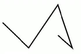
POLYLINE(19, XDK, YDK)
Fig. 1 Representation of polylines
2.2 POLYMARKER
Instead of drawing lines through a set of points, we may wish just to mark the set of points. GKS provides the primitive polymarker to do just this. A polymarker is generated by the function:
POLYMARKER (N, XPTS, YPTS)
where the arguments are the same as for the polyline function, namely XPTS and YPTS are arrays giving the N points (XPTS (1), YPTS (1)) to (XPTS(N), YPTS(N)). Polymarker places a centered marker at each point. GKS recognizes the common use of markers to identify a set of points in addition to marking single points and so the marker function is a polymarker.
The attributes that control the appearance of polymarkers are:
1. Marker, which specify one of five standardized symmetric characters to be used for the marker. The five characters are dot, plus, asterisk, circle and cross.
2. Marker size scale factor, which controls how large each marker is (except for the dot marker).
3. Polymarker color index which specifies what color the marker is.
Fig. 2 Polymarkers
2.3 TEXT
So far we have not attempted to put a title on our pictures. To do this, GKS has a text primitive which is used to title pictures or place labels on them as appropriate. A text string may be generated by invoking the function:
TEXT(X, Y, STRING)
where (X, Y) is the text position and STRING is a string of characters.
However, text is more complicated than the other primitives that we have examined. Everybody is used to good quality text in books whether it is the printed text of the book itself or text within the context of diagrams. Text is printed at different sizes, in different fonts, at different orientations and at different spacings. Graphics devices. on the other hand, are often not good at text; indeed some are not capable of text at all. Those that do often only have a restricted number of sizes. one or perhaps two orientations, and a single font. The attributes that control the appearance of text are:
1. Text font and precision, which specifies what text font, should be used for the characters and how precisely their representation should adhere to the settings of the text attributes.
2. Character expansion factor, which controls the height-to-width ratio of each plotted character.
4. Text color index, which specifies what color the text ring should be.
5. Character height, which specifies how large the characters should be.
6. Character up vector, which specifies at what angle the text should be drawn.
7. Text path, which specifies in what the text should be written (right,left,up or down).
8. Text alignment, which specifies vertical and horizontal centering options for the text string.
2.3 FILL AREA
There are many applications for which line drawings are insufficient. The design of integrated circuit layouts requires the use of filled rectangles to display a layer. Animation systems need to be able to shade areas of arbitrary shape. Other applications using colour only realize their full potential when they are able to use coloured areas rather than coloured lines.
At the same time, there are now many devices which have the concept of an area which may be filled in some way. These vary from intelligent pen plotters which can cross-hatch an area to raster displays which can completely fill an area with a single colour or in some cases fill an area by repeating a pattern.
GKS provides a fill area function to satisfy the application needs which can use the varying device capabilities. Defining an area is a fairly simple extension of defining a polyline. An array of points is specified which defines the boundary of the area. If the area is not closed (i.e. the first point is not the same as the last point), the boundary is the polyline defined by the points but extended to join the last point to the first point. A fill area may be generated by invoking the function:
FILL AREA (N, XPTS, YPTS)
where, as usual XPTS and YPTS are arrays giving the N points (XPTS(1), YPTS(1)) to (XPTS(N), YPTS(N)).
Let us extend our original set of data to describe a closed area. Nineteen data points were previously defined to which we add a further 24.
X 28.8 27.2 25.0 23.0 21.5 21.1 21.5 22.8 24.1
Y 12.3 11.5 11.5 11.5 11.2 10.5 9.0 8.0 7.0 5.1
X 25.2 24.2 22.1 20.0 18.0 16.0 14.0 12.0 10.0 8.0
Y 3.6 1.9 1.1 0.9 0.7 0.8 1.0 1.0 1.2 1.8 X 6.1 4.2 3.0 1.3
Y 2.1 2.9 4.1 6.0
Like the other primitives we have considered. Fill area has a representation accessed by a fill area attribute called the fill area index.
The fill area index is set by the function:
SET FILL AREA INDEX (N)
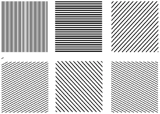
where N is the desired value of the fill area index. Filled areas may be distinguished by their filling style (called interior style in GKS) and colour. Let us assume that fill area representation 1 is interior style HOLLOW and that fill area representation 2 is interior style SOLID, each in standard colour. The filling style patterns used are given in the figure below:
Fig. 3 Pattern of Filling Area
III. CELL ARRAY
Fig. 4 Example illustrating GKS output primitives
IV. CONCLUSIONS
GKS is widely adopted for use in systems all over the world. The functions are defined independently of device type, application and programming language. Implementation of GKS in any programming language consequently remain device and application independent. The functionality of GKS is wrapped up as a data model standard in the STEP standard. Graphical application programs based on GKS thereby achieve device independent too.
REFERENCES
[1] Udit Agarwal, Computer Graphics, Bareilly, 2010. [2] http://ngwww.ucar.edu/gks/intro.html