Expert System-Based Predictive Cost Model for
Building Works: Neural Network Approach
*Amusan, L.M
1, Mosaku, T.O
2, Ayo, C.K
3, Adeboye, A.B
4Covenant University Ota, Nigeria.
[email protected], [email protected] , [email protected], [email protected].
Abstract
--
Project managers need accurate estimate of building projects to be able to choose appropriate alternatives for their constructions. Estimated costs of building projects, which hitherto have been based on regression models, are usually left with gaps for high margin of errors and as well, they lack the capacity to accommodate certain intervening variables as construction works progress. Data of past construction projects of the past 2 years were adjusted and used for the study. This model is developed and tested as a predictive cost model for building projects based on Multilayer Perceptron Artificial Neural Networks (ANNs) with Levenberg Marqua. This model is capable of helping professionals save time, make more realistic decisions, and help avoid underestimating and overestimating of project costs. The model is a step ahead of Regression models.Index Term-- Expert-S ystem, Predictive cost, Neural-Network, Cost, Model and Regression.
1 INT RODUCT ION
A number of uncompleted and abandoned projects are attributable to overall bad projects management of which poor forecasting approach is a factor. Poor cost forecasting approach will lead to underestimating or overestimating and
consequently cost overrun. Project abandonment as a result of cost overrun arising from poor cost forecasting approach, is
an interesting phenomenon locally as well as globally. This phenomenon has led to various stakeholders in built
environment to be aware of importance of accurate project cost right from conceptual stage of building project as well as throughout the life cycle of the project work. The awareness of working with accurate cost has thus created a trend among various clients including private, corporate, as well as public clients (government), that prudency in resources allocation is a great necessity for successful execution of project works. Thus in a bid to have an appreciation of what the project cost should be, clients resort to request for cost implications of various aspect of the project for purpose of planning, so also to have better appreciation of magnitude of project cost and environmental cost implication of the project as well as impact of the projects financial implication on client’s and other stakeholders decision. This development led to the advent of forecasting project cost so as to generate project cost information which reveals what the value of a project cost could be in future. However, in providing project cost information, cost estimator often resort to using traditional approach, recent developments on the other hand has proven the fact that traditional approach, which uses historical methods do not tend to capture the details of project works cost components, as well as intervening variables that impacts
the cost magnitude. Without gainsaying once the process is faulty, the end result could not be anything less to an
incomplete account of project’s cost and cost overrun. The cube method was the first recorded forecasting method;
this was invented about 200 years ago, floor area approach was developed around 1920 [1], some researchers later developed storey enclosure method on 1954, which provides better result over the previously developed cube and floor area, certain variables were identified and incorporated into the model other than those used in the past, like floor areas vertical positioning, storey heights, building shape and presence of basement.
However in the mid-1970s, researchers started deploying statistical techniques cost modeling, through these, conventional methods evolved, such as approximate quantities and optimization. Peculiar to the research work in this era is possibility of demonstrating the applicability of the developed models, as a result of seemingly non applicable nature of model generated.
1.1 DEFINIT ION OF COST MODEL
however, a cost model should be able to produce the cost implication, total cost, cost prediction for planning purpose, design evaluation, comparing design alternative and to forecast economic effects of changes in design and regulations.
2. RESEARCH FRAM EWORK
2.1 Emergence of New World Order in Cost Modeling The limitations identified with the conventional models stimulated the researchers not to rest on their oars, the drive to evolve better method then became the order of the day. The existing models then were not challenged since they lack applicability until advocators stressed the need to depart from existing research status -quo and go for research output that can be backed with solid theory. He doubts the reliability of existing forecasting models and urged the development of good forecasting method with solid framework for applicability [3].
The awareness of the need to shift research focus lead to the emergence of three (3) categories of forecasting models; the Black box and realistic models; Deterministic/Stochastic models and Deductive/inductive models
2.2 Deductive Verses Inductive Modeling
Models for purpose of cost prediction in construction can be cost categorized into deductive and inductive model, in form and structure. Data can be analyzed using design variables with a view to developing a mathematical relation that will described relationship among the variables and relate them to price, the type of model synthesized through this type of model is referred to as deductive model, it utilizes the system of correlation, least-square regression, such models arise largely from equation of this type:
P = fi(V1, V2, V3 …………..V
). Where P = the forecasted criteria, which are a function of f1, of the design variables, V1, V2, V3 …………..V
.Inductive model involves the synthesis of the cost of particular design solutions from design element or cost centers. The summation of cost centers and portfolio representing cost will yield the forecast price. Inductive models arise larg ely from the equation
P =
jn
j
j
C
f
1
Where P is the forecasted price, which is the sum of all committed resources; fj is the function of cost centres and project portfolio Cj, J equal 1to n, where n is the total number of project or cost series. Results are often calculated and aggregated and used as index of performance monitoring [3] [4].
2.3 Deterministic/Stochastic Modeling: Deterministic model assumes that values can be attributed to all variables, and that the variables can be determined and predicted exactly. Deterministic model can then be defined as a model without a formal measure of uncertainty; most of the models developed
are deterministic in nature since they are without formal measure of uncertainty. They produce single output; which is left at the mercy of forecaster to intuitively address [5][6]. Researchers in a bid to address the challenge of uncertainty associated with conventional model, developed the technique of embedding factor of coefficient of variation, to buffer the effect of variables’ lopsided dispersion; this is common in regression analysis; cumulative effect of data distribution is also used to buffer the effect of frequency disparity in Monte Carlo simulation analogy. The introduced buffer, helps eliminating the unwanted effect of data handling that can negatively impact the model output. [6].
2.4 Synthetic versus Product-based-models.
Synthetic approach to cost modeling is also referrered to as Blackbox approach. Cost of blackbox and realistic item, under synthetic approach is often obtained from the constituent elements, which is a function of design configuration. Components of building which had been systematically arranged following a pre-established configuration are often extracted and quantified using estimators’ specified technique. Thus, the cost obtained from such a method can be described as construction methodology dependent, and evolved out of the design, following builders construction methodology( an advance form of this is the popular builders estimate) [7]. Realistic models on the other hand are product-based. This type of model takes no account of configuration or details of design, but based on certain building parameters, such as: the floor area, volume of the proposed projects, users ’ parameters, among many others. [5]. Realistic approach attempts to represent the ways in which cost arise using finished product unlike synthetic approach this often makes it suitable at early and design stage, of building work.
3. CURRENT TRENDINMODEL DEVELOPM ENT Since the advent of storey enclosure method in mid -1950s, researchers had been laboring to bring to reality, an advance technique in cost modeling, for better result and quality output; manual approach was formerly in use, which was tedious and time consuming, since then other researchers have used different methods even till date when information technology had lead to emergence of new direction in cost estimating and forecasting.
3.1 Currently-used cost Estimation model
The breakdown of incidence of utilizing the modeling techniques is as follows:
TABLE ITRADITIONAL MODEL.
Modeling Average unit Average incidence-in-use Rank
Financial method 2.2 1%-33% 5
Superficial method 3.9 34%-36% 2
Superficial perimeter 2.2 34%-66% 7
Cube 1.8 0% 9
Storey enclosure 2.1 1%-33% 8
Approximate quantities 4.0 67%-99% 1
Elemental method 3.7 34%-66% 4
Bill of quantities 3.9 34%-66% 3
Source: [8]
TABLE II
NON TRADITIONAL COST FORECASTING MODEL
Modeling Average point Average incidence-in-use Rank
(i) Regression analysis 1.5 0% 4
(ii) Causal Model 1.5 0% 5
(iii) Monte Carlo simulation 1.5 0% 6
(iv) Value management 2.4 1%-33% 1
(v) Knowledge-based model 1.3 0% 7
(vi) Resource-based model 2.0 1%-33% 2
(vii) Life cycle cost model 1.7 0% 3
Source: [8]
The table indicated only value management resource-based model and lifecycle cost model as being widely used. Thus there has been little or no response to the paradigm shift as previously advocated by researchers. [9] called for shift in the
choice of non-traditional modeling approach over the old traditional modeling technique, this lead to the advent of non-traditional models presented in table III below with their incidence of use.
TABLE III
CURRENTLY-USED COST FORECASTING MODEL.
Modeling Average point Average incidence-in-use (IIU) Rank
Neural network 1.2 0% 2
Fuzzy logic 1.2 0% 3
Environmentally & sustainable development
1.6 0% 1
Source: [8]
To this end therefore this study developed a predictive cost model with a non-traditional method using neural network.
4. REVIEW RELAT ED WORKS ON NON-T RADIT IONAL MODELS( (NEURAL NET WORKS)
[10] carried out parametric cost estimating of highway projects using Neural Network, the purpose of the research is to provide an effective cost data management for highway projects in New Foundland. United Kingdom.
The study utilized the actual construction cost of 85 highway projects constructed cost estimating system for the projects in a modular architecture with several components
Back propagation was used as an optimum training interface to predict the outcome of new cases. So also, through the model developed, the effect of cost related parameters on the total cost of construction projects was determined through its sensitivity analysis.
However, the scope of the study did not include Building projects, it is limited solely to road construction projects while the preliminary test carried out on the extent of applicability of the model indicated that, the model can only be used at preliminary stage of project works, this limit the application to preliminary design stage where the acceptable level of accuracy is within 20% range.
To this end therefore, this study used data of completed building projects in Nigeria, since the location of the research is Nigeria , the costs was adjusted with Nigeria-based construction price index, to incorporate certain economic cost differential parameters.
105 different construction projects in Netherland that are not location dependent were used in this research work.
In another related study, [11] carried out a study on Neural Network application in solving actual cost problems in construction project. With reference to the outcome of the research work, feed forward Neural system was found to have the greatest r-value and followed in regression order by Radial basis function (RBF), Kohonen self organizatio n network (KSO), Recurrent Network, and simple recurrent network. The scope of the study did not include us ing the output in formulating the model; it was about using the output generated to select the best method with accurate output of which feed forward neural system was found to have best output, the accuracy of generated output was the parameter used to arrive at this conclusion.
So also, [3] carried out a research on application of Neural Network in predicting construction cost indexes. The work centered on estimating the changes in cost indexes better than those used in the past. 200 construction costs of 250 projects was used, with prime lending rate for the month, the year, was also used as input data into the neural network system. Exponential smoothing and linear regression were used as module for comparison of output generated.
The research concluded with a statement on the reliability of the output, that neural network produced a slightly poor prediction for changes in cost index. This is in dicative of the fact that variables affecting the construction cost indexes other than those used in the research need to be identified. However since the area of coverage of the study did not include modeling for holistic cost of the building other than constructions cost indexes, this research work is about achieving this feat; using multi-criteria cost approach. In the same vein, [12] estimated cost of Timber bridges using neural networks. The study deployed neural network and the output was simulated with output from regression analysis in order to determine which approach has least mean square error (r-square values). The study used cost parameters of the Timber Bridge such as volume of the web, volume of the decks and wooden flange bridge weight as neural network input data. The study with neural network indicated that, the r-square values using neural network system were greater than when regression analysis was used. So also, according to the researchers’ submission, in estimating the cost of timber bridges, the models with 3 – input variables gave the least error while the Neural network systems gave little variance between the actual cost and expected cost.
In the same context, [13] in their work, deployed Neural network versus parameter based application, and used neural network systems in carbon steel pipes cost estimating. 110 samples of carbon steel pipes were used for the study, with cost parameters such as pipe diameter, elbow and flange rating fed into the system: the system generated cost 1100fts as output. So also the same parameters were used as input in regression analysis, using multiple regressions. The outputs from both systems were compared to draw correlation among the outputs.
The study towed the line of submission as previous reviewed works did, in stating that mean square error generated using neural network system was less than mean square error obtained from multiple regression approach. The study concluded with stating that the neural network system is more accurate than the parameter based application.
The study area of coverage excluded model development as well as studying relationship among the input variables which this study is set to achieve. This study will use cost parameters of completed Building works as neural network input data and model development.
5. RESEARCH METHODOLOGY
The method used in carrying out the work is in two stages; the design stage, modeling stage (training stage) and the testing (validation) stage
5.1 The Design of Artificial Neural Network: Neural
network architecture and Back propagation learning technique were used in this study from Neurosolution software or Matlab. The proposed model was developed in three stages: the modeling stage, the training stage and the testing stage.
5.2 The Modeling Stage: This entails identification ofinput parameters using cost-significance work package (CSWP) and the adoption of Network architecture with its internal guide principles. This depends on factors such as the nature of problem, data characteristics, complexity of data and the number of sample data.
The hidden layer of the network with satisfactory number of processing elements (neurons) corresponding to the number of input layers (parameters) and one output layer of one processing element as target was chosen. A number of hidden layers were selected after several trials during training phase; this is basically determine by trials since there is no rule to determine it.
5.3 Data description: Cost significance work packages
models were used for this research. The concept involves combining similar items into packages that are similar in nature and correspond more closely to site operation than to the individual items. The work packages models are based on principle of cost-significance items with a base in Pareto principle. The principle is based on the assertion that 80% of the value of bill of quantities is contained within only 20% of the items, which are cost significant.
5.4 The Training Stage: The training data set (40 samples) was used to train the network, so as to select its parameters, the one suitable to problem at hand. Back propagation was used to train the network since it is recommended and simple to code. So also gradient descent momentum and learning rate parameters was set at the start of the training cycle (for speed determination and network stability, range of momentum 0.1
x
1, high = weight oscillation coefficient).develops the input to output, by minimizing a mean square error (MSE) cost function measured over a set of training examples. The M.S.E. is given by this relation:
M.S.E = [( square root of [[[summation). Sub. (i=1). Sup.n) [(xi – E (i)].sup.2]]]
n
Where n is the number of projects to be evaluated in the training phase, [X.sub.i] is the model output related to the sample, and E is the target output. The mean square error is an index of successfulness of a training exercise. The error was measured for each run of the epoch number selected; however training was stopped when the mean square error remains unchanged for a given number of epochs. This is to avoid
overtraining, and technical dogmatism when presented with an unseen example (data).
5.5 The testing phase: data from remain 10 samples were used as testing data set to produce output for unseen sets of data. A spreadsheet simulation program on Microsoft excel was used to test the generated model, according to optimized weights, comparison was made between actual cost and neural network cost, using cost percentage error (CPE) and mean estimated error (MEE).
CPE = [[Enn – Bv]/[Bv]]
100%MEE = [1n][[ I = n]. summation over (i = 1)] cpe(i)
TABLE I
BILL OF RESIDENTIAL CONSTRUCTION PROJECT FOR MODEL TESTING WITH EXTENSION P ERIOD OF 2008-2009
Project B. O. Q. Value (adjusted)
Actual B.O.Q. Value Variation Percentage (%) variation
1 30, 800 21,599 9, 201 42.59
2 42, 700 29,943 12,757 42.59
3 25, 000 17,532 7,468 42.59
4 15, 325 10,747 4,578 42.59
5 9, 251 6,488 2,763 42.58
6 16, 800 11,781 5,0819 42.60
7 28, 428 19,936 8,492 42.60
8 42, 534 29,828 12,706 42.60
9 40,101 28,121 11,980 42.60
10 67,247 47,158 20,089 42.60
Note: 5% Inflation factor and 10% Corruption escalator was factored into the B.O.Q value.
Legend:
Laspeyre price index
Index =
When lo = Base Index
li = Current year index wo = weighting woli = Indices B.O.Q. = Bill of quantity. P.V. = Percentage Variation.
In table I above, extracted cost values from bill of quantities were presented, the actual bill value and price index-adjusted cost, the variation ranges from N2.763m lowest value to
6. DATA ANALYSIS
N20.89m highest value after being adjusted. The adjusted value was used in validating and testing the model.
The system of derived price index used to adjust the bill cost value is Laspeyre price index as stated by the equation ab ove. Price index of year 2008 and 2009 were used, since bill of quantities used for the analysis were those of projects completed within the last two years. Also from the analysis, post adjustment percentage difference that exists among the project value range from 42.58 to 42.60 for lower to higher bill value.
TABLE II
NEURAL NETWORK OUTP UT AT MODEL TESTING P HASE
Project B.O.Q Value (B.V) N000,000m Predicted value (P.V) Nm
Variation (V) (B.V.-P.V.) Nm
Cost percent error (C.P.E.) (%)
1 30.800 29500 1300 +4.220
2 42.700 44100 -1400 -3.280
3 25000 25840 -840 -3.360
4 15325 15133 192 +1.330
5 9251 10101 -850 -9.190
6 16800 15125 -1149 +9.970
7 28428 29300 1675 -3.070
8 42534 42300 -872 +0.550
9 40101 41850 234 -4.36
Table II present the cost percentage and variation error of the developed model as new costs were presented of the test cases. The variation margin between the predicted value and actual bill value is between N0.84m lower limit to N1675m
upper unit, while cost percentage error oscillates between – 3.07% to =4.22% .
TABLE III
LEVEL OF ACCURACY EXP ECTED AT TRAINING P HASE
Model Maximum error (positive)
Maximum error (negative)
Mean error Standard deviation
Percentage accuracy
(%)
Neural network model output
+9.97 -9.19 0.39 6.240 5.85-6.53
A level of accuracy is expected at the testing phase, this is to ensure validity of the output generated. Therefore, table III contains the summary of error, standard deviation and range of expected accuracy. From the analysis extracted from table II,
maximu m expected negative error is -9.19 while maximu m positive error is +9.97. This generated mean error of 0.39, standard deviation of 6.24 percentage accuracy range is 5.85 to 6.53.
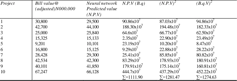
TABLE IV
CORRECTION ANALYSIS OF BILL VALUE AND NEURAL NETWORK- P REDICTED VALUE AT MODEL TESTING P HASE.
Project Bill value@ (adjusted)N000.000
Neural network Predicted value (N.P.V)
N.P.V (B.q) (N.P.V)2 (B.q.V)2
1 30,800 29,500 90.86x10⁷ 87.03x10⁷ 94.86x10⁷
2 42,700 44,100 188.30x10⁷ 194.48x10⁷ 182.33x10⁷
3 25,000 25,840 64.6x10⁷ 66.77x10⁷ 62.50x10⁷
4 15,325 15,133 2.35x10⁷ 22.90x10⁷ 23.49x10⁷
5 9,201 10,101 23.19x10⁷ 10.20x10⁷ 8.47x10⁷
6 16,800 15,125 9.29x10⁷ 22.88x10⁷ 28.22x10⁷
7 28,428 29,300 25.41x10⁷ 85.85x10⁷ 80.82x10⁷
8 42,534 42,300 83.29x10⁷ 178.93x10⁷ 180.91x10⁷
9 40,101 41,850 179.91x10⁷ 175.14x10⁷ 160.81x10⁷
10 67,247 66,128 444.7x10⁷ 437.29x10⁷ 452.22x10⁷
∑=1111.90 ∑=1281.47 ∑=1274.63
LEGEND:
N.P.V---Neura l Predicted Value B.Q.V---Bill of Quantity Value
The co-efficient of correlation using product moment approach
r =∑(B.q.V) (N.P.V) =1111.90 =1111.90
( ∑(N.P.V)2 √(1274.63)(1281.47) √1633400.1061
R (co-efficient of correlation = 0.87
In an attempt to study the strength of association existing among the parameters, product moment correlation was used. Correlation coefficient of 0.87 was obtained. This indicates high level of correlation and close association between the variable between actual bill cost and neural network predicted cost.
However, it is necessary to test the correlation by further statistical techniques, which relate the sample size and
probability levels. The following relation was used in further cross validation.
t = r √(n-2) when r = co-efficient of correlation. √ (1-r2) n = sample size
t = correlation test index. From analysis table IV, r = 0.87; n = 10
:. t = 0.87 √(10-2) √ (1-0.872) t = 4.99
This maps the outcome of the correlation test index (t) with t-tabulated value and degree of freedom v (8). The value of‘t’ above indicates highly significant correlation among the variables.
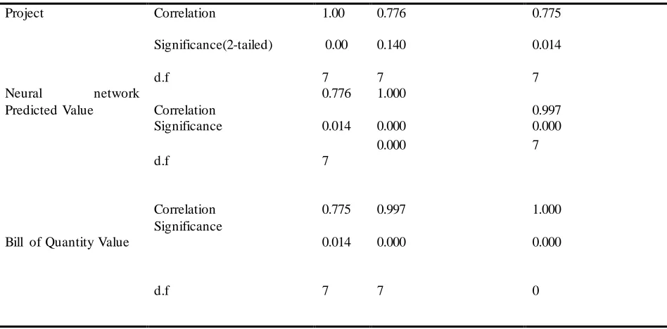
TABLE V
CORRELATION OF NEURAL NETWORK PREDICTED VALUES AND BILL VALUES USING NPV AS CONTROL VARIABLE.
Project Correlation 1.00 0.776 0.775
Significance(2-tailed) 0.00
0.140 0.014
d.f 7 7 7
Neural network
Predicted Value Correlation
0.776 1.000
0.997
Significance 0.014 0.000 0.000
d.f 7
0.000 7
Bill of Quantity Value
Correlation 0.775 0.997 1.000
Significance
0.014 0.000 0.000
d.f 7 7 0
Table V above present the correlation analysis of three variables, the result indicated that there is perfect correlation between the Neural network predicted value and the Bill of quantity value, the correlation index being less than 0.05 at 7.0 degree of freedom. Thus there is little or no variation from
the value predicted when the bill value was fed into the Neural network predictor and actual adjusted bill value, however variation factor was incorporated into the cost data used in the prediction.
TABLE VI
MODELS’ ATTRIBUTES USING NET PRESENT VALUE [NPV] AS MODELING PARAMETER M odel Fit statistics M ean Standard Error
M inimum M aximum
Stationary- R Square Value -0.144 0.084 -0.241
-0.940
R-Squared Value
0.412 0.104 0.345 0.532
Randomized Squared Error[RM SE]
9152.310 7924.940 2.102 13827.408 M aximum Percentage Error[M APE]
37.645 1.674 36.079 39.410
TABLE VII
SUMMARY OF NEURAL PREDICTED MODEL AND BILL MODEL
Model R_ Square Value Standard Estimate
Error
Significance Change
Bill Model
-0.241 0.450 0.000
Neural Network Predicted Value Model
-0.098 0.230 0.000
Table VI and VII present the characteristic feature of the model, maximum percentage error using the R-square value as index ranges from -0.241 to -0.940, 2.41 percent underestimate to 9.41 percent overestimate. This indicates 7.41 percent variation, between Bill value and Neural Network predicted value. The variation account for the corruption escalator factor and inflation factor built into the adjusted Bill value before being fed into the Neural machine.
7.0 CONCLUSION
The analysis carried out in the study, presents preliminary validation of prospect of obtaining a model that will predict building construction cost with minimum error, this also demonstrates the applicability of Neural network in forecasting the cost of building work. The result of the analysis indicates high level of accuracy in the output obtained from the neural network model with maximum variation factor of 7.42 percent. The corruption escalator factor and inflation buffer factored into the Bill value accounts for this variation. This indicates that in predicting value for subsequent project cost, the percentage can be factored into such cost to arrive at the actual cost value for such project. It is believed that the model will be suitable for use at different stages of project work
REFERENCE
[1] 1 Skitmore, R.M, and Ng, S.T .(2003)Forecast models for actual construction time and cost”, Building and Environment. Vol. 38, No 8, Pp 1075.
[2] 2 Hu M. Y; Shanker, M. and Hung, M. s. (2004). Predicting Consumer Situational Choice with Neural Networks. Anals of Operations research, 87, PP 213 – 232.
[3] 3 William, T .P. (2004). Neural Networks to Predict Construction Cost Indexes. In T opping, B.H.V., and Khan, A.I., Editors, Neural Networks and Combinatorial Optimization in Civil and Structural Engineering, Civil-Comp Press: 47-52.
[4] 4 Walczak S. (2004). Forecasting Emerging Market Indexes with Neural Networks. Journal of Managements Information System, 17(4), 203 -222.
[5] 5 Moore C.F; Lees, T . and Fortunes, C (1999) T he Relative Performance of Traditional and New Cost Models in strategic Advice for Clients. Rics paper series. London.
[6] 6 Adedayo, A.O; OjO, and Obamiro, J.K (2006) Operations Research in Decision analysis and Production Management.
[7] 7 Ferry, D.J; Bandon, P.S (2000) Cost Planning of Building. Blackwell
[8] Science Limited. 4th Edition. London.
[9] 8 Azmi A (2009) Cost Model in used for Industrialized Building Projects in Malasia
[10] Journal of Applied Sciences.Pp23-39
[11] 9 Brandon, A. (1987) Cost modeling for Estimating. T he Royal Institut ion of chartered surveyors, London.
[12] 10 Hegazy,T and Ayed, A.S. (1998). Parametric Cost Estimating of Highway Projects Using Neural Networks. Journal of Construction Engineering and Management, 124(3) 210 -225.
[13] 11 Copeland, J and Proudfoot, A (2000). Neural Networks T echniques in Solving Actual Cost Problems in Construction Projects. Journal of Construction Management and Engineering,ASCE, 123(2), 250 -270. [14] 12 Creese, R., and Li, L. (1995) Cost Estimation of T imber Bridges Using Neural Networks, Cost Engineering, AACE International, 37(2), 14-18.
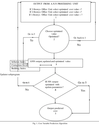
Choose optimized value Optimized?
2
Inflation Index Corruption Escalator Building Index
OUTPUT FROM A.N.N PROCESSING UNIT
If 3-Storeys Office Unit select optimized cost value =? If 2-Storeys Office Unit select optimized cost value =? If 1-Storeys Office Unit select optimized cost value = ?
1
Go back to 1
No
Go to 3
Ye
s
ANN output, updated and optimized value
3
IS NN output optimized with update parameters?
4
Output predicted cost
5 Updater subprogram
Go to 1