A Class of Shrinkage Testimators for the
Shape Parameter of the Weibull Lifetime Model
Zuhair A. Al-Hemyari
Ministry of Higher Education Oman
H. A. Al-Dabag Babil University, Iraq
Abstract
In this paper, we propose two classes of shrinkage estimators for the shape parameter of the Weibull distribution in censored samples. The proposed estimators are studied theoretically and have been compared numerically with existing estimators. Computer intensive calculations for bias and relative efficiency show that for, different values of levels of significance and for varying constants involved in the proposed estimators, the proposed testimators fare better than classical and existing estimators.
Keywords: Shape parameter; Censored data, Weibull failure model, Shrinkage, Preliminary test, Bias ratio, Relative Efficiency.
1. Introduction
The Weibull model (Weibull 1939, 1951, 1952) is often used in the field of life data analysis due to its flexibility. In addition, it can simulate the behavior of other statistical distributions such as the normal and the exponential. Indeed, the wide application and occurrence of the Weibull distribution in reliability engineering and in failure analysis are a wonder. Specific applications of the Weibull model are employed to represent manufacturing and delivery times in industrial engineering, to forecast weather data, to model fading channels in wireless communications, to exhibit good fit to experimental fading channel measurements, as well as in radar systems to model the dispersion of the received signals level produced by some types of clutters, etc. Other applications are studied by many other authors (see Lieblein and Zelen 1956, Kao 1959, Berrettoni 1964, Al-Mmeida 1999, Fok et. al. 2001, Erto and Pallotta 2007, and Rinne 2009).
1.1 The Model and Classical Estimator
Let ti, i1,2,...,n be a random sample of size n, from the two-parameter Weibull
distribution with probability cumulative distribution function,
) 1 ( 0,
0, , 0 t , )] / exp[-(t
-1 ) , |
F(t
Let y log te ; then y follows an extreme value distribution (refer to Bain 1972) with the probability distribution function,
) 2 ( ,
0 ,
-, y -, )] u)/ -y exp[-exp((
-1 ) , |
F(y u b b u b
whereb1/
and uloge are respectively the scale and the shape parameters.The estimations of the unknown parameters of the above model are quite complicated. Bain and Engelhardt (1992) have proposed a simple estimation procedure of the reciprocal of the shape parameter as follows. Let
) , m ( )
2 ( ) 1
( t ... t
t and y(1) y(2) ... y(m) be the m smallest ordered
observations in a sample of size n from (1) and (2) respectively. Define an unbiased estimator forbas,
) 3 ( )],
( [ ) / 1 ( ) , ( ), (
, /
ˆ 1
1 1
1
m i m
i m
i m
i
W W E
n n
m k y y T
m T
b
where Wi (yi u)/b, i1,2,...,m, are ordered variables from the extreme value distribution with b1 and u0, mnk(m,n) and k(m,n), being unbiased constants, represent the ratio ofmton; some values of k(m,n)are given in White (1967), and Engelhardt and Bain (1973). The statistic T(bˆ)2bˆ/b2T/b (Bain 1972), has been shown to follow chi-square distribution with 2m degrees of freedom. The p.d.f. of T is given by,
) 4 ( otherwise.
0,
0, , 0 T , )] T/ (m))exp[-( /
T { ) | f(T
1
-
b b b
b
m m
Therefore, we have ˆ(m1)/T, E(ˆ) and MSE(ˆ|)2/(m2).
1.2 Incorporating a prior value, and Shrinkage
When a life testing experimenter becomes familiar with failure data, knowledge is developed concerning the parameters of the model. The discipline of quality control deals with setting the process to a suitable average on the basis of control charts. Since the mean of the Weibull failure time depends on the shape parameter, a similar control method can be used to bring the shape parameter to some prefixed value (0),leading to improvement in the performance of an item or component, i.e., reducing the MSE of the new estimators or it may give a saving in sample size. Indeed, the prior information costs time and money; and incorporating such prior information in the estimation of the unknown parameters is also utilizes the past cost of sampling units.
(ii) we fear that 0 may be near the true value of , i.e., something bad
happens if 0
and we do not know about it.In both cases, the value 0 is available, and in such a situation, it is natural to
start with an estimator
ˆ of
and modify it by moving it closer to 0, so that the resulting estimator, though perhaps biased, has a smaller mean squared error than that of
ˆ in some interval around 0. This method of constructing an estimator of
that incorporates the prior information 0 leads to what is known as a shrunken estimator. It may be recalled that Thompson (1968) the first who proposed the shrinkage estimator, which suggests the use of a prior point guess of the parameter for improving the performance of the existing estimator
ˆ. Al-Hemyari and Al-Al-Hemyari and Ali (2010, 2012)have proposed some shrinkage testimators for the scale parameter and reliability function of the Weibull model.The purpose of this paper is not simply to extend to extend our previous testimators (2010, 2012) to the shape parameter of the Weibull model. Rather, we assume a censored sample where the aim is to find some testimators of the shape parameter which offer some improvement over the classical and similar estimators. Assuming the scale parameter is known, two appropriate choices of exponential type shrinkage weighting functions are used and the expressions for the bias, mean squared error, and relative efficiency of the proposed testimators are derived, studied and compared numerically.
2. Shrinkage estimators
Define the class of Huntsberger (1955) type shrinkage estimator for the shape parameter
by,) 5 ( },
))
ˆ
( 1 (
ˆ
)
ˆ
( { ~
0
where(ˆ) (0(ˆ)1),represents a weighting function specifying the degree of belief in 0.
The shrinkage estimator of the shape parameter
has been considered by several authors (Singh and Bhatkulikar 1977, Pandey 1983, Pandey, et. al. 1989, Pandey and Singh 1993, and Singh and Shukla 2000). Estimator (5) is also studied for the shape parameter
but in different contexts (Singh et. al. 2002). It may be noted here that other authors (e.g., Kambo et. al. 1990, 1992, Parkash et. al. 2008, and Al-Hemyari et. al. 2009, 2011) have tried to develop new shrinkage estimators of the form (5) for special populations by choosing different weight functions.It is also noted that the performance of these estimators strongly depends on the choice of (ˆ).If (ˆ) is not set in accordance with reality (i.e., large (ˆ)when
o
either there is no significant gain in the performance of ~ or there is actually a significant loss.
2.1 Bias and MSE of
~The bias of
~ by definition is,) 6 ( )],
ˆ
))(
ˆ
( 1 [( )
~ ( ) | ~
( E E 0 B
whereB(ˆ|)0,is the bias of
ˆ. The mean squared error (MSE) expression of
~ is given by,) 7 ( )], ))(
ˆ ( 1 [( ) ( 2 ] ) ˆ )( ) ˆ ( 1 [( ) | ˆ ( )
~ ( ) | ~
( 2 0 0
0 2
2
E MSE E E
MSE
where MSE(ˆ|),is the mean squared error expression of
ˆ. When 0 we have) 8 ( .
0 ] )
ˆ
)( )
ˆ
( 1 [( )
|
ˆ
( )
| ~
( 0 2
2 0
0
MSE E
MSE
Remark1:
i) Non-negativity: Clearly, the proposed class of estimators {~:0(ˆ)1} is
a convex combination of
ˆ and 0, hence
~
is always positive.
ii) Unbiasedness: Based on equation (6), if (ˆ)1, or
ˆ
0 with probability one, the proposed estimator turns into the unbiased estimator, otherwise it is biased. Thus, we conclude the following: There does not exist any unbiased estimator of
in the class of estimators{~:0(ˆ)1} except the above undesirable cases.iii) Minimum mean squared error estimator: It is not easy with the type of the proposed testimator to establish the minimum mean squared error biased estimator, i.e.,MSE(~|)MSE(ˆ|), for every (ˆ) and every
with strict inequality for at least one
. But when 0 the inequality holds (seeequation (8)), this means that by a proper choice of (ˆ), the proposed
shrinkage estimator performs better (in the sense of smaller MSE) than
ˆ in the neighborhood of 0.2.2 The Shrinkage estimator 1
~
The first proposed testimator for
of the class {~:0(ˆ)1} is denoted by 1~ and uses the unbiased estimator ˆ1 (m1)/T and the following modified
shrinkage weight function,
) 9 ( 0 , 1 0 , 1 ) ˆ ( 0
1
c a e a cmT
Using (6) and (7), the bias ratio (bias/
) and mean squared error expression of1
~
are given respectively by,
) 10 ( , ) 1 ( ) 1 /( [ ) / ) | ~ ( ( 1 1
a cm m cm m
B
) 11 ( )]}, ) 1 /( )( 2 ( )) 1 /( ) 2 (( 2 ) 1 )[( ) 1 /( ( )] ) 1 /( ) 2 (( )) 1 /( ) 1 )( 2 (( ) 1 )[( ) 1 /( ( 2 1 ){ ˆ ( ) | ~ ( 2 2 2 2 2 2 1 cm m cm m m cm a cm m cm m m cm a MSE MSE m m
where(0 /).The relative efficiency of 1
~
is denoted by Eff(~1;ˆ1|) and given by, ) 12 ( )]}. ) 1 /( )( 2 ( )) 1 /( ) 2 (( 2 ) 1 )[( ) 1 /( ( )] ) 1 /( ) 2 (( )) 1 /( ) 1 ( ) 2 (( ) 1 )[( ) 1 /( ( 2 1 /{ 1 ) | ~ ( / ) | ˆ ( ) | ˆ ; ~ ( 2 2 2 2 2 2 1 1 1 1 cm m cm m m cm a cm m cm m m cm a MSE MSE Eff m m
2.3 The Shrinkage estimator 2
~ Since the shrinkage estimator 1
~
is biased, in this section, in place of unbiased estimator ˆ1, we will use the biased estimator ˆ2 ((m2)/(m1))ˆ1, in (5)
denoting the resulting estimator by 2
~
with the weight function
) 13 ( . 0 , 1 0 , 1 ) ˆ
( ( 1) 0
2
c a e
a cm T
Again using (6) and (7), the bias ratio (bias/
) and mean squared error expression of ~2 are given respectively by) 14 ( )), 1 /( 1 ( ]] ) ) 1 ( 1 )( 1 /[( ) 2 ( ) ) 1 ( 1 /( [ ) / ) | ~ ( ( 1
2
m m c m m m c a
) 15 ( )]}. ) ) 1 ( 1 /( )( 1 ( )) ) 1 ( 1 /( ) 2 (( 2 ) 2 )[( ) ) 1 ( 1 /( ( )] ) ) 1 ( 1 /( ) 1 (( )) ) 1 ( 1 /( ) 1 )( 2 (( ) 2 )[( ) ) 1 ( 1 /( ( 2 1 ){ | ˆ ( ) | ~ ( 2 2 2 2 2 2 2 2 m c m m c m m m c a m c m m c m m m c a MSE MSE m m
The efficiency of ~2 relative to ˆ2 is given by,
) 16 ( )]} ) ) 1 ( 1 /( )( 1 ( )) ) 1 ( 1 /( ) 2 (( 2 ) 2 )[( ) ) 1 ( 1 /( ( )] ) ) 1 ( 1 /( ) 1 (( )) ) 1 ( 1 /( ) 1 )( 2 (( ) 2 )[( ) ) 1 ( 1 /( ( 2 1 /{ 1 ) | ˆ ; ~ ( 2 2 2 2 2 2 2 2 m c m m c m m m c a m c m m c m m m c a Eff m m
The efficiency of 2
~
relative to ˆ1 is given by,
) 17 ( ). | ˆ ; ˆ ( )) 2 /( ) 1 (( ) | ˆ ; ~
(2 1 m m Eff 2 2
Eff
Remark 2: Consistent estimator. Since lim (~ | )0,
i
n B and | ) 0,
~ (
lim
i n MSE 2
1 i i, , ~
are asymptotically unbiased and consistent estimators.3. Preliminary Shrinkage estimators
In section 2, a class of Huntsberger type shrinkage estimator was studied, and two cases for the shape parameter with known scale parameter were discussed by using two different shrinkage weight functions and two different classical estimators. This section also deals with the estimation of the shape parameter of the Weibull distribution with known scale parameter, where we developed a preliminary test shrinkage estimator when its initial estimate 0 is given.
Shrinkage estimators
~i, i1,2 have the disadvantage of necessarily using the prior value in the construction of final estimators. However, it is not necessary that the prior value be close to the true value. To employ this idea in the estimation of the shape parameter
of the Weibull distribution, a preliminary test is first conducted to check the closeness of 0 to
before using it in ashrinkage estimator. If the preliminary test is accepted, (ˆ)(ˆ0)0 is used
as an estimator of
; otherwise
ˆ itself is taken as an estimator of
. Thus, the proposed testimator is taken as one of two alternatives depending on this test. To satisfy this idea, setwhere (ˆ)(0(ˆ)1).The class of preliminary shrinkage estimators (PSE) with this weight function is denoted by ~p and given by,
) 19 ( },
]
ˆ
[ ] )
ˆ
)(
ˆ
( {[ ~
0
0 R R
p I I
where IR and IR are respectively the indicator functions of the acceptance region
R and the rejection region R. The relevance of such types of shrinkage estimators lies in the fact that, though they may be biased, they have smaller MSE than
ˆ in some interval around o.It may be denoted here that the class of estimators (19) is a special case of the class (5).It may be noted here that the class of preliminary test shrinkage estimators p ~
is
completely specified if the shrinkage weight factor(ˆ) and the region R are specified. Consequently, the success of ~ now depends upon the proper choice
of (ˆ) and R. In general, the true value of
is unknown, i.e., (ˆ) should not be a function of unknown
and hence, a proper choice of (ˆ)cannot be guaranteed. Similarly for the choice of region R there is no unified approach.3.1 Bias and MSE of p ~
The bias and mean squared error expressions of ~p are derived for any ˆ, (ˆ) and R and given respectively by:
) 20 ( ,
) | ( )]
ˆ
))(
ˆ
( 1 [( )
; | ~
( R 0 f T dT
B
R
p
) 21 ( .
) | ( )]
ˆ
))(
ˆ
( 1 [( ) ( 2
) | ( ] ) )( )
ˆ
( 1 [( ) |
ˆ
( )
; | ~ (
0 0
2 0 2
dT T f
dT T f MSE
R MSE
R R p
When 0 we have:
) 22 ( ,
) | ( )]
ˆ
))(
ˆ
( 1 [( )
; | ~
( 0 R 0 f T 0 dT
B
R
p
) 23 ( .
) | ( ] ) )( )
ˆ
( 1 [( ) |
ˆ
( )
; | ~
( 2 0
0 2
0
0 R MSE f T dT
MSE
R
p
Remark 3: From equations (22) and (23) above, it may be noted that remark 1 derived in section 2, is also valid for the shrinkage estimator~p, i.e., the unbiasedness and minimum mean squared error estimator properties are valid when using PSE. This means that there does not exist, any unbiased estimator of
in the class of estimators ~p(0(ˆ)1), except the same undesirable3.2 Choices for region R
As was noted earlier, the performance of the class of estimators (19) depends on a proper choice of the region R and the shrinkage function (ˆ). Having chosen
),
ˆ
(
in this section, we now discuss the criterion for choice of the region R.It seems reasonable to construct a region R, denoted by R1, by the criterion,
) 24 ( )},
| ˆ ( )
( :
{ 0 2 0
1
a MSE
R
where a0 is constant to be chosen such that MSE(~p |0)is minimum. Then
1
R simplifies to:
) 25 ( },
,
ˆ ˆ
)], ) 1 /( ) 1 ( 1 ( ); ) 1 /( ) 1 ( 1 ( , 0 max( [
,
ˆ ˆ
], ) 1 /( 1 ( ; ) 1 /( 1 ( , 0 [max( {
2 0
0 1
2
1 0
0 1
1
1
if m
m a m
m a R
if m
a m
a R
R
where ˆ1 and ˆ2 are defined in sections 2.2 and 2.3 respectively. The second choice of R, we consider the commonly used acceptance region of the hypothesis H0 : 0 against the alternative H1: 0. If
is the level of significance of the test, then the preliminary test region R1is given by,) 26 ( ]},
, [ ) ˆ (
{T
L1 /2 U/2R
where L1/2 and U/2are the lower and upper 100(
/2) percentile points of thestatistic T(ˆ) used for testing the above hypothesis. If the chi-square statistic
ˆ ) 2( 1)ˆ /
( 1 m 1
T (or T(ˆ2)2(m2)ˆ2 / ) is used, the region R2 is given by,
) 27 ( },
, ˆ ˆ ), , ))
2 ( 2 / [(
, ˆ ˆ ), , ))
1 ( 2 / [( {
2 2
2 , 2 / 1 0
) 2 ( 2 2
1 2
2 , 2 / 1 0
2 1 2
if m
R
if m
R R
m m
where 2 2 , 2 / 1 r
is the lower 100(
/2) percentile point of the chi-square distribution with 2m degrees of freedom. In this section, two testimators for the shape parameter
of the Weibull distribution, when a prior guess value of the shape parameter is available from the past with known scale parameter, will be discussed.3.3 The PSE~p1
The first proposed testimator for
of the class {~p :0(ˆ)1} is denoted by1
~ p
and uses the unbiased estimator ˆ1 (given in section 2.2) and with the
shrinkage weight function (ˆ ) 1 a e c(m)T 0,0 a 1,c 0,
1
if
ˆ1Ri. Let, b a ], b , a [
expressions for the bias ratio and mean squared error of
1
~ p
are obtained as follows: ], ) 1 ( 2 / )) , ;( 1 ( ) 1 ( 2 / )) , ;( ( [ ) / ) ; | ~ (
( 1 1
1 1 1 1 1
m m
i i m m i i i j
p R a G m a b cm G m a b cm
B
(28) ) 29 ( )]}, ) 1 ( 2 / )) , ( ; ( )( 2 ( ))) 1 ( 2 / 1 ( )) , ( ; 1 ( ) 2 (( ) 2 / )) , ( ; 2 ( ) 1 )[(( ) 1 /( ( ))] 1 ( 2 / )) , ;( ( ) 2 (( )) 1 ( 2 / )) , ;( 1 ( ) 1 ( ) 2 (( ) 2 / )) , ;( 2 ( ) 1 )[(( ) 1 /( ( 2 1 ){ ˆ ( ) ; | ~ ( 2 2 2 2 1 2 2 2 2 2 2 2 1 1 1 1 1 2 1 1 2 1 cm b a m G m cm b a m G m b a m G m cm a cm b a m G m cm b a m G m b a m G m cm a MSE R MSE m i i m i m i i m m i i m i i m i i m i j p
where 1a1
0(1 a/m2)(
1 Cm), 2b1
0(1 a/m2)(
1 Cm),), 2 )( 2 / 1 ( ), 2 )( 2 / 1
( 1 2 1 0 1
0 1
2a a m Cm b a m Cm
, ), 2( 1 1 2 2 2
2 ) 2 , 2 / ( 0 2
2
b b Cm
a
m
and( / 2) 1 / 2
( )
( ; ( , )) exp( / 2) , 1, 2, 1, 2. (30)
( / 2)2
j i
j ii
b q
i
i j i j i q
a
y
G q a b y dy j i
q
The efficiency of
1
~ p
relative to ˆ1 is given by,
) 31 ( )]}}. ) 1 ( 2 / )) , ( ; ( )( 2 ( ))) 1 ( 2 / 1 ( )) , ( ; 1 ( ) 2 (( 2 ) 2 / )) , ( ; 2 ( ) 1 )[(( ) 1 /( ( ))] 1 ( 2 / )) , ;( ( ) 2 (( )) 1 ( 2 / )) , ;( 1 ( ) 1 ( ) 2 (( ) 2 / )) , ;( 2 ( ) 1 )[(( ) 1 /( ( 2 1 /{{ 1 ) ; | ˆ ; ~ ( 2 2 2 2 1 2 2 2 2 2 2 2 1 1 1 1 1 2 1 1 2 1 1 cm b a m G m cm b a m G m b a m G m cm a cm b a m G m cm b a m G m b a m G m cm a R Eff m i i m i m i i m m i i m i i m i i m i j p
3.4 The SPE
2
~ p
In section 3.3, the SPE is studied based on ˆ1. In this section, in place of the unbiased estimator ˆ1, we will study the SPE based on the biased estimator
, / ) 2 ( ˆ
2 m T
with the weight function (ˆ ) 1 a e c(m 1)T 0,0 a 1,c 0,
2
if i R 2 ˆ
and denoting the resulting testimator by ~ .2
p
Let Rj [jai,jbi]. Again using equations (20) and(21), the bias ratio (bias/
) and mean squared error expression of2
~ p
are given respectively by:
) ( )]}, ) ( ) /( )) , ( ; ( ) ( ( ))) ) ( ( / ))( , ( ; ( ) ( ) /( )) , ( ; ( ) )[( ) ) ( /( ) (( )))] ) ( ( ) /( ))( , ;( ( ) (( )) ) ( ( / )) , ;( ( )( )( ( ) / )) , ;( ( )[( ) ) ( /( ) ( ){ | ˆ ( ) ; | ~ ( 33 cm 1 2 2 m b a m G 1 m 1 m c 1 2 1 b a 1 m G 2 m 2 b a 2 m G 2 m 1 m c 1 2 m a 1 m c 1 2 2 m 1 b a m G 1 m 1 m c 1 2 b a 1 m G 1 m 1 2 b a 2 m G 1 m c 1 1 m a 2 1 MSE R MSE 2 m i 2 i 2 2 1 m i 2 2 2 m i 2 i 2 2 m 2 m i 1 i 1 1 m i 1 i 1 2 m i 1 i 1 2 m 2 i j p2
where 1a1 max(0,0(1 f)(1 C(m1))), 2b1 0(1 f)(1C(m1)),
)), 1 ( 2 )( 1 ( )), 1 ( 2 )( 1
( 1 2 1 0 1
0 1
2
m C f b m C f
a
, )),
1 ( 2
( 1 1 2 2 2
2 ) 2 , 2 / ( 0 2
2
b b m
C
a
m
andf a(m2)/(m1).The efficiencyof ~p2 relative to ˆ2 is given by,
) 34 ( )]}. ) 1 ( 2 ) 2 /( )) , ( ; ( ) 1 ( ( ))) ) 1 ( 1 ( 2 / 1 ))( , ( ; 1 ( ) 2 ( ) 2 /( )) , ( ; 2 ( ) 2 )[( ) ) 1 ( 1 /( ) 2 (( )))] ) 1 ( 1 ( 2 ) 2 /( 1 ))( , ;( ( ) 1 (( )) ) 1 ( 1 ( 2 / )) , ;( 1 ( )( 1 )( 1 ( ) 2 / )) , ;( 2 ( )[( ) ) 1 ( 1 /( ) 1 ( 2 1 /{ 1 ) ; | ~ ( 2 2 2 2 1 2 2 2 2 2 2 2 1 1 1 1 1 2 1 1 2 2 cm m b a m G m m c b a m G m b a m G m m c m a m c m b a m G m m c b a m G m b a m G m c m a R Eff m i i m i m i i m m i i m i i m i i m i j p
The efficiency of
2
~ p
relative to ˆ1 is given by,
) 35 ( ). ; | ˆ ; ~ ( )) 2 /( ) 1 (( ) ; | ˆ ; ~
( p2 1 jRi m m Eff p2 2 jRi
Eff
4. Simulation and Numerical Results
The bias ratio and relative efficiency of
~i, i1,2 and ~ , i1,2i
p
were
computed for different values of the constants involved in these estimators. The following numerical results and comparisons are based on these computations.
4.1 Numerical Results of
~i :For the testimators
~i, i1,2 numerical computations computed for ,20
. 1 , 5 . 0 , 1 . 0 , 05 . 0 , 01 . 0 , 001 . 0
a In tables1-4, some sample values of the relative
efficiency, and in tables 5 and 6, some values of bias ratio are given for some selected values of n,m,a andc.
i) It was observed from the computations that generally
, 2 , 1 ), |
ˆ
; ~
( i
Eff i i increases asc decreases.
ii) For fixedc, the relative efficiency increases slightly as a decreases (from 1) when 0.5
1.6.iii) The relative efficiency is a concave function of , with the maximum at ,
1
a1, c0.004; where for other values of a and c the relative efficiency is not a concave function of
.iv) The relative efficiency is an increasing function with m, i.e., the relative efficiency is higher for the heavy censoring (n 20,m3) than for other censoring (n20,m5,8).
v) The testimators
~i, i1,2 are biased (see tables 5 and 6). The bias ratio is reasonably small, in the neighborhood of
1.In addition, the bias ratio of1
~
is generally smaller than that of ~2, and hence the computations of bias ratio of 2
~
are not reported here for space consideration.
vi) From the computations of relative efficiency given in tables 1-4, as expected the shrinkage estimators give higher relative efficiency in some region around o. It is observed that the estimators , 1,2
~
i i
have a smallermean squared error than the classical single stage estimator
ˆ for the effective interval (broader range of |
| for which efficiency is greater than unity)0.1
5,whena1, andc0.5. For the choice a1, c0.005, the mean squared error is much smaller than the classical estimator (as much as 494 times form3), but the effective interval decreases to 0.5
1.7.Thus,
~i, i1,2 may be used to improve the efficiency if the ratio 0/ is expected to belong to the above effective intervals.vii) It is seen that the relative efficiency ~2 is much higher than that of ~2 whena1, c0.005 and o is sufficiently close to
. In fact for, 5 . 0 ,
1
c
a and 0.1
3 both estimators will give almost the same order of efficiency (tables 1-6).4.2 Numerical Results of pi ~
For the estimators ~ , i1,2,
i
p
the computation was done for
, . , . , . ,
.0100501015 0
1 , 5 . 0 , 1 . 0 , 05 . 0 , 01 . 0 , 001 . 0
a and 0.1(0.1)2(1)5.some sample values of the relative efficiency are given in Tables 7-14, and some values of the bias ratio are given for some selected values of n,m,a andc.
i) It is observed from our computations given in tables 9-16, that the relative efficiency of ~ , i1,2
i
p
decreases with size
of the pretest region, i.e., 01. 0
gives higher relative efficiency than for other values of
.ii) Both regions Rj, j 1,2 give a smaller mean squared error for , 1,2 ~
i
i
p
than the classical estimator for the intervals 0.1
1, 0.1
2 respectively when a0.5, c0.004 and decreases otherwise.iii) It is observed from our computations given in tables 7-12 for fixed
and c that the relative efficiency of ~ , i1,2i
p
is a concave function with a0.5.
iv) It is also seen that from Tables 7-12, for fixed a,c and , the relative efficiency of ~ , i1,2
i
p
is a decreasing function of m.
v) The region R2 yields higher relative efficiency than R1, for both ~ , i 1,2
i
p
and hence the computations of bias ratio and relative efficiency of
i
p
~ whenR1 is used, are not reported here for space consideration.
vi) It is seen that the relative efficiency of
2
~ p
is much higher than that of
1
~ p when
1.vii) It is observed that the testimators ~ , i1,2
i
p
are biased. The bias ratio of
1
~ p
is reasonably small for all values ofm,a,c and
(tables13 and 14).4.3 Comparisons
Comparing results of
~i, i1,2 given in tables 1-4 with the tables given in (Singh and Bhatkulikar 1977, Pandey 1983, Pandey, Malik, et. al. 1989, Pandey and Singh 1993, and Singh and Shukla 2000), it is seen that our proposed testimators are better both in terms of higher relative efficiency and for the wider range of
for which efficiency is greater than unity. It may be noted here that the numerical results of Singh and Shukla (2000) were calculated for the values of (/0)(1/)0.54.0, which are equivalent to (0 /)0.252, in ourcomputations. In addition, comparing results of testimators ~ , i1,2
i
p
given in
tables 7-14 with the above existing results, it is seen that our testimators compare favorably.
5. Conclusions
estimator ~ have been suggested. The performance of the proposed shrinkage estimators of the shape parameter when some prior guess value of
is available have been analyzed by using the criteria of bias ratio, mean squared error and relative efficiency. The class of estimators thus obtained seems to be an improved version of the existing estimators given in subsection 4.3, subject to certain conditions. The proposed estimators lead us to formulate many interesting estimators of shrinkage type. It is identified that when the guessed value 0 coincides exactly with the true value
and also when 0 is moderately far away from ,we get a larger gain in efficiency over the classical estimator in the effective interval of (broader range of
for which efficiency is greater than unity). Thus, even if the experimenter has less confidence in the guessed value, the efficiency of the proposed estimators can be increased considerably by suitably choosing the scalars a,c and
. The suggested estimators have substantial gain in efficiency for a number of choices of a,c and , when the sample size is small i.e., for the heavy censoring (n20,m3). Even for large sample sizes, so far as the proper selection of scalars is concerned, all the proposed estimators are found more efficient than the classical estimator but for a smaller effective interval of
.The superiority of the suggested estimatorsp
~ over the existing estimators given in subsection 4.3 has also been recognized. The suggested class of shrinkage estimators are therefore recommend for its use in practice.
References
1. Al-Hemyari, Z. A. and Ali, A. R. (2012). Shrinkage techniques for estimation in Weibull lifetime Distribution. Submitted for publication.
2. Al-Hemyari, Z. A. Husain, I. H. and Al-Jebory, A. N. (2011). A class of efficient and modified testimators for the mean of normal distribution using complete data. I. J. of Data analysis Techniques and Strategies, 3, 4, 406-425.
3. Al-Hemyari, Z. A. (2010). Some testimators for the Scale parameter and Reliability Function of Weibull Lifetime Data”, J. of Risk and Reliability, 224, 197-205.
4. Al-Hemyari, Z. A., Kurshid, A., and Al-Gebori, A. (2009). On Thompson testimator for the mean of normal distribution. Investigacion Operacional, 30, 109-116.
5. Al-Mmeida, J. B. (1999) Application of Weibull statistic to the failure of coating. J. of Material Processing Technology, 93, 257-263.
6. Bain, L.J., and Engelhardt. M. (1991). Statistical Analysis of Reliability and Life Testing Models. Marcel Dekker, New York, NY.
7. Bain, L. J. (1972). Inferences based on censored sampling from the Weibull or Extreme value distribution. Technometrics, 14, 693-703.
9. Engelhardt, M. and Bain, L.G. (1973). Some complete and censored sampling results for the Weibull and Extreme- value distribution. Technometrics, 15, 541-549.
10. Erto, P. and Pallotta, G. (2007). A new control chart for Weibull technological processes, Quality Technology and Quantitative Management, 4, 553-567.
11. Fok, S. L., Mitchell, B. G., Smart, J. and Marsden, B. J. (2001). A numerical study on the application of the Weibull theory in brittle materials. Engineering Fracture Mechanics, 68, 1171-1179.
12. Harris, E. and Shakarki, G. (1979). Use of the population distribution to improve estimation of individual mean in epidemiological studies. J. of chronic disease, 32, 233-243.
13. Huntsberger, D.V. (1955). A generalization of a preliminary testing procedure for pooling data. Ann. Math. Statist. 26, 734-743.
14. Kao, J. H. K. (1959). A graphical presentation of mixed Weibull parameters in life- testing electron tubes. Technometrics, 4, 309-407. 15. Kambo, N.S. Handa, B.R. and Al-Hemyari, Z.A. (1990). On shrunken
estimators for exponential scale parameter. J. of Statistical Planning and Inferences, 24, 87-94.
16. Kambo, N.S. Handa, B.R. and Al-Hemyari, Z.A. (1992). On Huntsberger type shrinkage estimator. Communications in Statistics- Theory and Methods, 2(3), 823-841.
17. Lieblein, J. and Zelen M. (1956). Statistical investigation of the fatigue life of deep groove ball bearings. Journal of Res. Nat. Bur. Std., 57, 273-315. 18. Pandey, M. (1983). Shrunken estimators of the of Weibull shape
parameters in censored samples. IEEE Transaction in Reliability, 32, 200-203.
19. Pandey, B. N., Malik, H. J. and Srivastava, R. (1989). Shrinkage testimators for the shape parameter of Weibull distribution under type II censoring. Communication in Statistics- Theory and Method, 18, 1175-1191.
20. Pandey, M. and Singh, U. S. (1993). Shrunken estimators of the of Weibull shape parameters from type-II censored samples. IEEE Transaction in Reliability, 42, 81-86.
21. Parkash, G., Singh, D.C., and Sinha, S.K. (2008). On shrinkage estimation for the scale parameter of Weibull distribution. Data Science J. 7, 125-136.
22. Parkash, G., and Singh, D.C. (2009). A Bayesian shrinkage approach in Weibull type-II censored data using prior point information. REVESTAT-Statistical Journal, 2:171-187.
23. Rinne, H. (2009). The Weibull Distribution A Hand book. A Chapman & Hall Book-Taylor & Francis Group.
24. Singh, H.P., Saxena S., Jack Allen, Singh, S. and
Randomness and Optimal in Data Sampling. Books.google.com. Arxiv.org. 1-20.
25. Singh, J. and Bhatkulikar, S.G. (1977). Shrunken estimation in Weibull distribution. Sankhya, B39, 382-393.
26. Singh, H.P., and Shukla, S. K.(2000). Estimation in the two- parameter Weibull distribution with prior information. IAPQR Transactions. 25, 107-118.
27. Sinha, S.K. (1986). Reliability and Life Testing. Wiley Eastern Limited. 28. Thompson, J. R. (1962). Some shrinkage techniques for estimating the
mean. J. Amer. Statist. Assos. 63, 113-123.
29. Weibull, W. (1939). A statistical theory of the strength of materials. Ingeniors Vetenskaps Akademiens Handingar, Royal Sweden Institute for Engineering Research, Stockholm, Sweden, No.151.
30. Weibull, W. (1951). A statistical distribution function of wide applicability. J. of applied mechanics, 18, 293-297.
31. Weibull, W. (1952). Discussion: A statistical distribution function of wide applicability. J. of applied mechanics, 19, 233-234.
32. White, J.S. (1967). The moments of Log-Weibull order statistics. General Motors Research Publication. GMR 717, General Motors Corporation, Warren, Michigan.
Appendix
Table1: ShowingEff (~1;ˆ1 |) when a=1 and c=0.005
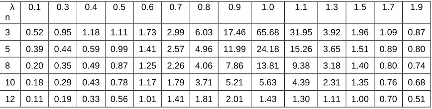
Table 2: Showing Eff (~1;ˆ1 |) when a=1 and c=0.5
λ n
0.1 0.3 0.4 0.5 0.6 0.7 0.8 0.9 1.0 1.1 1.3 1.5 1.7 1.9 3
3 1.31 1.34 1.41 1.39 1.35 1.31 1.27 1.24 1.21 1.18 1.142 1.12 1.09 1.09 1.07
5 1.25 1.29 1.28 1.24 1.20 1.17 1.14 1.10 1.09 1.07 1.05 1.04 1.02 1.01 1.01
8 1.23 1.22 1.20 1.16 1.15 1.13 1.10 1.09 1.07 1.05 1.03 1.01 1.01 1.00 1.00
10 1.21 1.20 1.17 1.15 1.14 1.12 1.09 1.08 1.07 1.05 1.02 1.00 1.00 1.0 1
12 1.16 1.15 1.14 1.13 1.12 1.11 1.07 1.06 1.05 1.03 1.00 1.00 1 1 1
λ n
0.1 0.3 0.4 0.5 0.6 0.7 0.8 0.9 1.0 1.1 1.3 1.5 1.7 1.9
3 0.52 0.95 1.18 1.11 1.73 2.99 6.03 17.46 65.68 31.95 3.92 1.96 1.09 0.87
5 0.39 0.44 0.59 0.99 1.41 2.57 4.96 11.99 24.18 15.26 3.65 1.51 0.89 0.80
8 0.20 0.35 0.49 0.87 1.25 2.26 4.06 7.86 13.81 9.38 3.18 1.40 0.80 0.74
10 0.18 0.29 0.43 0.78 1.17 1.79 3.71 5.21 5.63 4.39 2.31 1.35 0.76 0.68
Table3: Showing Eff(~2;ˆ2 |) when a=1 and c=0.005
Table4: Showing Eff(~2;ˆ2 |) when a=1 and c=0.5
λ n
0.1 0.3 0.4 0.5 0.6 0.7 0.8 0.9 1.0 1.1 1.3 1.5 1.7 1.9 3 5
3 2.37 3.99 3.81 3.21 2.69 2.32 2.06 1.86 1.73 1.61 1.46 1.36 1.29 1.24 1.11 1.04
5 2.16 2.21 1`.98 1.79 1.64 1.50 1.47 1.35 1.24 1.18 1.19 1.08 1.04 1.02 1.00 1.00
8 1.87 1.98 1.85 1.62 1.45 1.38 1.24 1.18 1.14 1.06 1.04 1.01 1.00 1.00 1.00 1
10 1.71 1.43 1.37 1.25 1.19 1.12 1.09 1.05 1.03 1.01 1 1 1 1 1 1
12 1.19 1.07 1.04 1.02 1.01 1.00 1 1 1 1 1 1 1 1 1 1
Table 5: Showing (B(~1|)/) when a=1 and c=0.5
λ n
0.1 0.3 0.5 0.7 0.8 0.9 1.0 1.1 1.3 1.5 1.7 1.9 3
3 -.60 -.26 -.13 -.07 -.05 -.04 -.03 -.03 -.02 -.01 -.01 -.00 -.00
5 -.30 -.05 -.01 -.00 -.00 -.00 -.00 -.00 -.00 -.00 -.00 -.00 -.00
8 -.11 -.00 -.00 -.00 -.00 -.00 -.00 -.00 -.00 -.00 -.00 -.00 -.00
10 -.03 -.00 -.00 -.00 -.00 -.00 -.00 -.00 -.00 -.00 -.00 -.00 -.00
12 -.00 -.00 -.00 -.00 -.00 -.00 -.00 -.00 -.00 -.00 -.00 -.00 -.00
Table 6: Showing (B(~2 |)/)when a=1 and c=0.5
λ n
0.1 0.3 0.5 0.7 0.8 0.9 1.0 1.1 1.3 1.5 1.7 1.9 3
3 -.67 -.45 -.38 -.36 -.35 -.34 -.34 -.34 -.33 -.33 -.33 -.33 -.33
5 -.39 -.22 -.20 -.20 -.20 -.20 -.20 -.20 -.20 -.20 -.20 -.20 -.20
8 -.21 -.14 -.14 -.14 -.14 -.14 -.14 -.14 -.14 -.14 -.14 -.14 -.14
10 -.13 -.11 -.11 -.11 -.11 -.11 -.11 -.11 -.11 -.11 -.11 -.11 -.11 λ
n
0.1 0.3 0.4 0.5 0.6 0.7 0.8 0.9 1.0 1.1 1.3 1.5 1.7 1.9
3 0.63 1.04 1.43 2.06 3.21 5.63 12.14 41.28 494.12 68.61 7.18 2.57 1.32 0.92
5 0.46 0.75 0.95 1.11 1.73 3.02 6.33 18.46 71.68 30.95 4.42 1.66 1.09 0.87
8 0.22 0.49 0.55 1.01 1.31 2.27 4.56 10.91 22.08 14.46 3.45 1.46 1.01 0.81
10 0.17 0.32 0.47 0.95 1.15 1.99 3.76 7.16 9.81 7.38 2.78 1.39 0.97 0.77
12 -.09 -.09 -.09 -.09 -.09 -.09 -.09 -.09 -.09 -.09 -.09 -.09 -.09
Table 7: Showing Eff(~p1;ˆ1 |;1R2)when a=1, c=0.005, n=20, β0 = 1 and α =0.01
λ n
0.1 0.2 0.3 0.4 0.5 0.6 0.7 0.8 0.9 1 2 3 4
3 2.502 2.104 2.017 1.963 1.915 1.864 1.809 1.751 1.691 1.629 1.039 .657 .446
5 1.143 1.145 1.142 1.136 1.128 1.118 1.106 1.092 1.078 1.062 .877 .728 .643
8 1.018 1.019 1.019 1.019 1.018 1.017 1.016 1.014 1.012 1.009 .981 .959 .954
Table 8: Showing Eff(~p1;ˆ1 |;1R2) when a=0.5, c=0.005, n=20, β0 = 1 and α =0.01
λ n
0.1 0.2 0.3 0.4 0.5 0.6 0.7 0.8 0.9 1 2 3 4
3 3.064 1.643 2.516 2.431 2.360 2.294 2.232 2.173 2.116 2.062 1.586 1.225 .967
5 1.518 1.405 1.299 1.278 1.264 1.250 1.237 1.223 1.210 1.197 1.075 .981 .919
8 1.119 1.046 1.044 1.041 1.039 1.036 1.034 1.031 1.029 1.026 1.007 .994 .989
Table 9: Showing Eff(~p1;ˆ1 |;1R2)when a=0.1, c=0.005, n=20, β0 = 1 and α= 0.01
λ n
0.1 0.2 0.3 0.4 0.5 0.6 0.7 0.8 0.9 1 2 3 4
3 1.189 1.173 1.167 1.162 1.159 1.155 1.151 1.148 1.144 1.141 1.107 1.069 1.032
5 1.063 1.061 1.059 1.057 1.054 1.052 1.050 1.048 1.045 1.043 1.024 1.007 .999
8 1.012 1.011 1.011 1.010 1.009 1.008 1.008 1.008 1.007 1.006 1.003 1 .999
Table 10: Showing (~ ; ˆ1| ;2 2)
2 R
Eff p when a=1, c=0.005, n=20, β0 = 1 and α =0.01
λ n
0.1 0.2 0.3 0.4 0.5 0.6 0.7 0.8 0.9 1 2 3 4
3 3.632 3.023 2.897 2.731 2.612 2.521 2.424 2.331 2.252 2.120 1.135 .552 .348
5 1.926 1.329 1.321 1.308 1.291 1.271 1.249 1.225 1.199 1.173 1 .712 .598
8 1.159 1.134 1.124 1.113 1.099 1.052 1.039 1.028 1.022 1.019 .996 .961 .941
Table 11: Showing Eff(~p2;ˆ1|;2R2)when a=0.5, c=0.005, n=20, β0 = 1 and α =0.01
λ n
0.1 0.2 0.3 0.4 0.5 0.6 0.7 0.8 0.9 1 2 3 4
5 2.068 1.721 1.396 1.360 1.385 1.320 1.305 1.280 1.255 1.211 1.082 1 .994
8 1.251 1.148 1.115 1.093 1.054 1.037 1.036 1.033 1.031 1.029 1.018 1 .992
Table 12: Showing (~ ; ˆ1| ;2 2)
2 R
Eff p when a=0.1, c=0.005, n=20, β0 = 1 and α =0.01
λ n
0.1 0.2 0.3 0.4 0.5 0.6 0.7 0.8 0.9 1 2 3 4
3 1.188 1.173 1.167 1.163 1.159 1.155 1.151 1.148 1.144 1.141 1.108 1.078 1.049
5 1.063 1.061 1.059 1.056 1.054 1.052 1.050 1.047 1.045 1.043 1.023 1.007 1
8 1.012 1.011 1.010 1.010 1.009 1.009 1.008 1.008 1.007 1.006 1.002 1 1
Table 13: Showing (B(~p1 |;1R2)/) when a=0.5, c=0.005, n=20, β0= 1 and α =0.01
λ n
0.1 0.2 0.4 0.5 0.7 0.8 0.9 1 2 3 4
3 -.112 -.101 -.090 -.090 -.080 -.070 -.067 -.061 -.001 .050 .090
5 -.031 -.030 -.021 -.021 -.021 -.011 -.011 -.010 -.000 .001 .011
8 -.001 -.001 -.000 -.000 -.000 -.000 -.000 -.000 -.000 .000 .001
Table 14: Showing (B(~p2 |;2R2)/)when a=0.5, c=0.005, n=20, β0= 1 and α =0.01
λ n
0.1 0.2 0.4 0.5 0.7 0.8 0.9 1 2 3 4
3 -.552 -.549 -.537 -.531 -.519 -.513 -.507 -.501 -.445 -.395 -.357
5 -.272 -.270 -.267 -.263 -.262 -.260 -.259 -.257 -.245 -.235 -.230