Computation of Sample Mean Range of the
Generalized Laplace Distribution
Kamal Samy Selim
Department of Computational Social Sciences
Faculty of Economics and Political Science, Cairo University
Cairo, Egypt
Abstract
A generalization of Laplace distribution with location parameter
,
, and scale parameter0,
is defined by introducing a third parameter
0
as a shape parameter. One tractable class of this generalization arises when
is chosen such that 1/
is a positive integer. In this article, we derive explicit forms for the moments of order statistics, and the mean values of the range, quasi-ranges, and spacings of a random sample corresponded to any member of this class. For values of the shape parameter
equals1
/ ,
i i
1,...,8
, and sample sizes equal 2,3,…,15 short tables are computed for the exact mean values of the range, quasi-ranges, and spacings. Means and variances of all order statistics are also tabulated.Keywords: Generalized Laplace distribution, Order statistics, Range, Quasi-ranges,
Spacings, Multinomial expansion.
1. Introduction
The probability density function of Laplace distribution with location parameter
,
, and scale parameter
0
, takes the form
1
( )
exp
,
.
2
x
f x
x
(1.1)
This distribution is also known in the literature as the double exponential distribution.
Laplace distribution has been extensively studied since its early introduction by Laplace
in (1774). For extensive reviews of this distribution and its statistical properties we refer
the reader to Johnson
et al.
(1995) and Kotz
et al.
(2001).
One possible generalization of Laplace distribution is to introduce a shape parameter
,
0
. In such case, the probability density function (1.1) takes the form (Kotz
et al.
2001)
1/ 1
1
1
( )
exp
,
,
2
(1 /
)
x
f x
x
And the cumulative distribution function
F x
( )
, can be easily derived as follows. For
,
x
1/ 1
1
1
( )
( )
.
2
(1/ )
x x
x
y
F
x
f y dy
e
dy
On setting
(
y
) /
/
t
, and with simple manipulation we get
1
1
1
( )
,
,
2
1 /
x
x
F
x
(1.3)
where
1( , )
tt
e dt
is the complementary incomplete gamma function. Similarly,
for
x
,
the cumulative distribution function takes the form
1
1
1( ) 1
( )
1
,
.
2
1 /
α
x
x
x
F
x
f y dy
(1.4)
Evidently, when
1
, the p.d.f. (1.2) yields the classical Laplace distribution (1.1), and
by varying the value of
, the model can better fit data with sharper peaks and heavier
tails. The generalized Laplace distribution can therefore be viewed as a flexible model
able to cope with empirical deviations from the Laplace model.
One interesting class of (1.2) is when the shape parameter
is assumed to be equal to
1
/ ,
i i
1,2, ...
, i.e., when
1 /
is a positive integer value. As it is known that when
is
a positive integer,
( , )
can be expanded as a finite summation (Gradshteyn and
Ryzhik
2007)
1
0
( , )
( )
.
!
i
i
e
i
Accordingly, under the assumption that
1 /
is a positive integer, the cumulative
distribution function of the generalized Laplace distribution function (1.3) and (1.4) can
be expressed as
1 (1/ ) 1
0
1 (1/ ) 1
0
1 1
2
1 1
2
1
1
for
,
!
( )
1
for
.
!
i x
i
i x
i
x
x
e
x
i
F x
e
x
i
Let
X
1
,
X
2
, ...,
X
n
be independent and identically distributed as generalized Laplace
distribution under the previously stated assumption about the parameter
.
Further, let
1 2
...
nX
X
X
be the corresponding order statistics of a random sample of size
( 2)
n
arranged in ascending order of magnitude. For any integer
r
,
2
r
n
/ 2
where
is the largest integer value less than or equal
,
the difference
, 1: 1
;
r n r n n r r
R
X
X
namely the distance between the
r
thvalues from either end of the
ordered sample, is known as the
r
thsymmetric quasi-range. Conventionally, when
r
1,
the difference
R
1, :n n
X
n
X
1is called the sample range. Also, of special interest are the
successive differences of order statistics
(
X
r1
X
r),
r
1,...,
n
1
referred to as the
sample spacings (David and Nagaraja 2003).
The sample range, the symmetric quasi-ranges, and the spacings and their linear
combinations have many theoretical uses and applications in statistical inference. For
excellent surveys of their theoretical uses we refer the reader to (David and Nagaraja
2003, Arnold 2008). Applications of order statistics, in general, and the sample range and
quasi-ranges, in particular, in estimation and tests of hypotheses are extensively surveyed
in (Harter and Balakrishnan 1996, 1998). (For an early survey of such applications, see
also (Chu 1957). Use of sample quasi-ranges in estimating population standard deviation
is studied by Masuyama (1957), Harter (1959), and Leone
et al.
(1961). David and
Nagaraja (2003) indicated the uses of spacings in building nonparametric and
sime-parametric confidence intervals for the population parameters, and Ahsanullah
et al.
(2013) covered their uses in quantile estimations. The generalized Laplace distribution on
the other hand, is employed in Bayesian inference and modeling (Taylor 1992), and its
applications in communications, economics, engineering, and finance are extensively
surveyed in (Kotz
et al.
2001).
Using the expressions of the density and distribution functions in (1.2) and (1.5),
respectively, exact explicit forms for the density function of the
thr
order statistic
, r 1,...,
r
X
n
, and the
ths
moment of
X
rabout the location parameter ,
are derived in
the next section. The means of the range, quasi-ranges,
and spacings of samples taken
from the distribution under consideration are the subject of section 3. Computational
aspects and directions on statistical applications of the derived means are considered in
section 4. The computed tables for samples of sizes 2,3,…,15 are given in the appendix.
2. Moments of order statistics
The following two propositions derive the probability density function of the
thr
order
statistic
X
r, and the
thProposition 2.1
Let
X
r(
r
1,..., )
n
be the
thr
order statistic of an i.i.d. random sample of size
n
( 1)
from the generalized Laplace distribution (1.2) under the assumption that
1 /
is a
positive integer. Then, the p.d.f. of
X
rdenoted by
f x
r( ),
is
(1/ ) 1
0
0 (1/ ) 1
1 ( )
(1/ ) 1 1/ 1 0 1 0 1/ 1 1 /
( 1) (
1)!
,
,
2
(
)
!( !)
( )
i i i i p k x r k n r k r pk p p k r
i i r
x
n n r
r r k n r r
k r
e
x
p i
f x
(1/ ) 1
0
0 (1/ ) 1
1 ( 1) 1
(1/ ) 1 1 1 0 0 1 1 1 /
( 1) (
)!
e
,
,
2
(
)
!( !)
i i i i p k xk n r r
k n r
p
k p p k n r
i i
x r
k
k n r
x
p i
(2.1)
where
p p
0,
1,...,
p
(1/ ) 1are non-negative integer values.
Proof: The probability density function of the
thr
order statistic is given by
1
!
( )
( )
( )
1
( )
,
(
1)!(
)!
n r r
r
n
f x
f x F x
F x
x
r
n
r
(2.2)
10
( )
( 1)
( )
.
n r
k k r k
n n r
r
r
f x
kF x
Hence, if
x
,
then substituting from (1.2) and (1.5) for
f x
( )
and
F x
( )
, respectively,
we get
1 1( ) (1/ ) 1
, 1/ 1
0 0
1
1
1
( )
.
(1/ )
2
!
k k r
x i
k r n r
r x k r
k i
n n r
r
r k x
f
x
e
i
(2.3)
Now, by the multinomial expansion of the finite power summation (Bender and
Williamson 2006), it could be easily proved that
0 1 0
0 1 0 1
0 1
0 0 1
0
!
!
,
!
!
!
! 0!
1!
!
!( !)
S i S i i S S i pm p p p
i S
S
S
p
i p p p m S p p p m
i i
y
m
y
y
y
y
m
i
p
p
p
S
p i
(2.4)
where m,
m p p
, ,
0 1,...,
p
Sare non-negative integer values.
Similarly, by expanding
1 (1
F x
( ))
r1, (2.2) could be written as
1
0
1
( )
( )
1
1
( )
.
r
k k n r r
k
n r
r
r k
f x
f x
F x
(2.5)
Hence, for
x
,
by substituting from (1.2) and (1.5) in (2.5), and following similar
steps as before, we reach the lower right hand side of (2.1).
Deriving the distribution function of
X
ris a straightforward exercise involving simple
variable transformations and some algebraic manipulation. The resulting distribution
comprises two functions of finite series of the complementary incomplete gamma
function.
Proposition 2.2
Under the same stated assumptions of proposition 2.1, the
ths
moment about the location
parameter
,
of the order statistic
X
r,
denoted by
(
)
r
s X
E
x
is given by
1/
1
1 1
0 0
1
1
1
(
)
,
(1 /
)
2
2
r
s k s k
n r r
s
X k r k r k n r k n r
k k
n n r r
r
r k k
E
x
G
G
(2.6)
Where for the non-negative integer values
p p
0,
1,...,
p
(1/ ) 1 the term
G
k r 1is given by
(1/ ) 1 0 (1/ ) 1
0
(1/ ) 1
0
1 (1/ ) 1
1/ ( 1) 1
0
1 /
(
1)
(
1)!
,
! ( !)
(
)
i i
i
i i k r
p i p s
p p k r
i i
i p
s
k r
G
p
i
k r
(2.7)
and
G
k n r is similarly given by (2.7) but with (
k n r
)
in place of (
k r
1)
.
Proof: Consider the
ths
central moment of the
thr
order statistic,
0
, 0 , 0
0
(
)
( )
( )
.
r
s s s
X r x r x
E
x
x f
x dx
x f
x dx
(2.8)
After substitution from (2.1), and making the change of variable
y
x/
/
, i.e.
1/ 1/
x
y
and
dx
1/1y
1/1dy
, the first integral in (2.8) yields
1/
0
, 0
0
1
( )
(1 /
)
2
s k s
n r s
r x k r
k
n n r
r
r k
x f
x dx
(1/ ) 1
0
0 (1/ ) 1
1/ ( 1) 1 ( )
(1/ ) 1
1 0
0
(
1)!
! ( !)
i i i
i p s
k r y
p
p p k r
i i
k
r
e
y
dy
p
i
1/
1 0
1
,
(1 /
)
2
s k s
n r
k r k r
k
n n r
r
r k
G
(2.9)
where
G
k r 1is given by (2.7).
Similarly, by substitution for
f
r x, 0( )
x
from (2.1), and the variable change, the second
integral in (2.8) gives
1/
1
, 0 1
0 0
1
1
( )
(1 /
)
2
s k
r s
r x k n r k n r
k
n r
r
r k
x f
x dx
G
,
(2.10)
where
G
k n r is as given by (2.7) but with
(
k n r
)
in place of
(
k r
1)
.
The proof is
then concluded by the substitution from (2.9) and (2.10) in (2.8).
Corollary 2.1: On setting
1,
we get the
ths
moment about the location parameter
of the
thr
order statistic connected with a sample of size
n
( 1)
from the classical
two-parameter Laplace distribution (1.1) as
( 1) ( 1)
1
1
0 0
1
1
(
)
1 (
1)
! !
(
)
(
1)!(
)!
2
2
r
k s s k s
n r r
s s
X k r k n r
k k
n r r
k
k r
kk n r
n s
E
x
r
n r
(2.11)
This same result appeared in Johnson
et al.
(1995, p. 168) but with an excessive
multiplication by
2
1.
3. Means of sample range, quasi-ranges, and spacings
In the early beginning of the last century, Pearson (1902) proved that the expected value
of the sample spacings takes the form
1
(
r r)
( )
r1
( )
n r,
1,...,
1.
n r
E X
X
F x
F x
dx
r
n
(3.1)
By summing both sides of (3.1) for all successive spacings from
r
r
1to
r
r
21
,
1 2
1
r
r
n
, we get
2 2
2 1
1 1
1 1
1
(
)
(
)
( )
1
( )
.
r r
r n r
r r r r
r r r r
n r
E X
X
E X
X
F x
F x
dx
(3.2)
The left hand side of (3.2) represents the mean of the difference between any two order
statistics
2
r
X
and
1
r
X
. Setting
r
1
1
and
r
2
n
,
and making use of the binomial
theorem, we get the known form of the sample mean range derived by
Tippett (1925)
1, :(
1)
1
( )
1
( )
.
n n
n n n
E R
E X
X
F x
F x
dx
Now, since
F x
( )
n
1
F x
( )
n
1
at x
, (3.3) could be written as
1, :
( )
1
( )
( )
1
( )
.
n n
n n
n n
E R
x F x
F x
F x
F x
dx
(3.4)
Applying the integration by parts reversely on (3.4), we get
1
1
1, :
( )
1
( )
( ) .
n n
n n
E R
xn F x
F x
f x dx
(3.5)
Another approach to derive (3.5) is to consider the difference between means of the two
extreme order statistics
X
nand
X
1
1
11, :
(
)
(
1)
( )
( )
1
( )
( ) .
n n
n n n
E R
E X
E X
xn F x
f x dx
xn
F x
f x dx
(3.6)
The following theorem states the derivation of explicit forms for the exact mean values of
the range, quasi-ranges, and spacings of a random sample taken from the generalized
Laplace distribution.
Theorem 3.1
Let
X
1
X
2
...
X
nbe the order statistics of a random sample of size
n
( 2)
drawn
from the generalized Laplace distribution (1.2) under the condition that 1/
is a positive
integer. Then, the mean difference
2 1
, 1
1 2 r rE X
X
r
r
n
is given by
0 0
2
2 1
1 1
(1/ ) 1
1
+
1
2
2
k k
n r r
k r k n r
k r k n r
k k
r r r
r r
n r r
k k
M
M
n
E X
X
r
,
(3.7)
where for the non-negative integer values
p p
0,
1,...,
p
(1/ ) 1the term
M
k ris given by
(1/ ) 1 0 1 (1/ ) 1
0 (1/ ) 1
0
1 (1/ ) 1
0
1
(
)!
!( !)
(
)
k r
i i i
i i
p p p k r i p
p i i
M
k r
i p
p i
k r
,
(3.8)
and
M
k n r is similarly given by (3.8) but with (
k n r
)
in place of (
k r
)
.
Proof: Recalling (3.2), it is true that
2
2 1
1 1
(
)
( )
1
( )
( )
1
( )
r
r n r r n r
r r
r r
n
E X
X
F x
F x
dx
F x
F x
dx
r
2
1 1
0 0
1
( )
11
( )
.
r n r r
k r k n r
r r k k
n n r k r k
r k
F x
dx
kF x
dx
Consider the first integral in (3.9), by substituting for
F
(
x
)
;
x
from (1.5), and
making the change of variable
y
1 /
(
x
) /
we get
(1/ ) 1 (1/ ) 1 ( ) (1/ ) 10 0
( )
.
2
!
k r i
k r y k r
k r i
y
F x
dx
e
y
dy
i
(3.10)
Applying the multinomial expansion (2.4) on the finite power summation in (3.10) then
gives
(1/ ) 1
0
0 1 (1/ ) 1
1 1 (1/ ) 1
( ) (1/ ) 1
0 0
(
)!
( )
.
2
!( !)
i i
i
i p
k r y k r
k r
p
p p p k r
i i
k r
F x
dx
e
y
dy
p i
(3.11)
With the change of variable
z
y
/ (
k
r
)
, the integral in (3.11) is clearly a gamma
function, and so
( )
(1/ ) 1
M
2
k r
F x
dx
k r
k r
,
(3.12)
where
M
k ris as given by (3.8).
Similarly, the second integral in (3.9), after substituting for
F
(
x
)
;
x
from (1.5),
making the change of variable
y
1 /
(
x
) /
, and applying expansion (2.4)
yields
(1/ ) 1
0
0 1 (1/ ) 1
1 1 (1/ ) 1
( )
(1/ ) 1
0 0
!
1
( )
.
2
!( !)
i i
i
i p
k n r y k n r
k n r
p
p p p k n r
i i
k n r
F x
dx
e
y
dy
p i
And with the change of variable
z
y
/ (
k
n r
)
, we get
1
( )
(1/ ) 1
M
2
k n r
F x
dx
k n r
k n r
,
(3.13)
where
M
k n r is given by (3.8) but with
(
k n r
)
in place of
(
k r
)
.
Finally, the substitution from (3.12) and (3.13) in (3.9) completes the proof of the
theorem.
Corollary 3.1: The following are straightforward consequences of theorem 3.1
1.
Setting
r
1
1
and
r
2
n
in (3.7) gives the mean of the sample range.
2.
Setting
r
1
m
and
r
2
n m
1
;
2
m
n
/ 2
, in (3.7) gives the mean of the
th
m
symmetric quasi-range.
3.
Finally, setting
r
2
r
11
in (3.7) gives the mean of the spacing
1 1 1
(
X
r
X
r)
;
1
Corollary 3.2: For
n
3, and
r
1
1,..., (
n
1) / 2
1,
the following relation is true
n r1 1 n r1
r1 1 r1
.
E X
X
E X
X
(3.14)
Poof: Set
r
1
1,..., (
n
1) / 2
1 and
r
2
r
11,
and then substitute in (3.7) to get both
sides of (3.14), the equality of the two sides becomes evidently true.
Corollary
3.3:
On
setting
1
we
get
the
mean
difference
r2 r1
, 1
1 2
E X
X
r
r
n
connected with a sample of size
n
( 2)
from the classical
two-parameter Laplace distribution (1.1) as
2
2 1
1
1 1
1
0 0
1 (
)
1 (
)
(
)
.
2
2
k k
r n r r
r r k r k n r
r r k k
n r r
k
k r
kk n r
n
E X
X
r
(3.15)
Remark 3.1: The explicit from (3.7) does not depend on the location parameter
,
. Not only is this so, but the dependence on the scale parameter
,
0
is especially simple multiplicative one. Hence, for example, if instead of the sample range
1, :n n
R
, we consider
W
1, :n n
R
1, :n n/
, then
E R
1, :n n
E W
1, :n n. Since, in this case the form of
1, :n n
W
, is independent of
,
and
, a single table suffices for the means of the range, for
each sample size, and each value of
.
4.
Computation algorithm and tabulation
Apart from the precision matters of computing large factorials and gamma functions, the
main difficulty in programming the derived forms (2.6) and (3.7) is the generation of all
possible terms of the involved multinomial expansions. The following algorithm provides
a straightforward approach to overcome this difficulty.
4.1 The compositions algorithm
Following the basic number theory concepts of partitions and compositions (See
Andrews 1976, Knuth 1997, Stojmenovic 2008), by partitions of a positive integer
m
into
z
parts, we mean all possible sets of
z
nonnegative integers that sum up to
m
.
Compositions are merely partitions in which the orders of the summands are taken into
account. Generating all of the decompositions of a nonnegative integer
m
into
z
nonnegative integers, is the same as to generate all of the possible
z
1
subsets of
1
m
z
objects.
The following algorithm; in Pascal-like notation, is adopted to generate all of the
compositions needed for computing summation like (3.8).
0
1/ 1
0 1 1
(
1,2,..., (1 /
) 1)
;
;
1;
0
;
1
1;
1;
;
0;
- 1;
1
i
h h h h
i
p
k
r t
k
r h
p
While p
k
r do
If t
then h
h
h
t
p
p
p
t
p
p
A Fortran 95 code, running on a Windows-based Intel® 3.00GHz CPU is written to
conduct all computations. The Fortran language provides better control over the precision
and accuracy of the computations. Interfacing this Fortran code with R is now under
consideration by the author besides other computational routines attributed to the
Generalized Normal and the multinomial distributions.
4.2 Tabulation
Given that the sampling distribution is the generalized Laplace (1.2) with parameters
1
and
equals
1, 1 / 2 ,..., 1 / 8
respectively, exact mean values of the range,
quasi-ranges, and spacings, as well as means and variances of all order statistics are computed
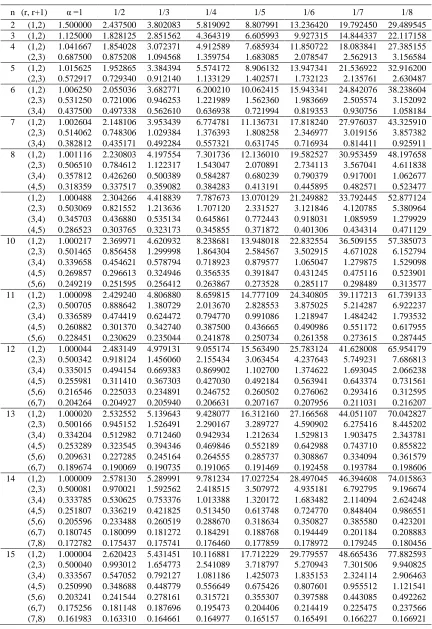
for samples of sizes equal to 2,3,…,15. Table 1 in the appendix gives the means of ranges
and quasi-ranges, and table 2 gives the means of the corresponding lower order spacings.
It should be noted that, for any sample size
n
3
, the identity relation (3.14) eliminates
the need to compute the means of the
(
n
1) / 2
higher order spacings, i.e., the means
of spacings not appeared in table 2, can be obtained by symmetry. Means and variances
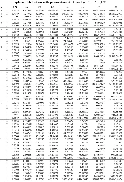
of higher order statistics are listed in tables 3 and 4, respectively. Again, there is no need
to list the means and variances of the lower order statistics, as it can be obtained using the
relation
E
(
X
r)
E
(
X
n r 1)
,
r
n
/ 2
, and for any odd sample size,
E
(
X
n/21) 0
.
Of special interest is the case when
1,
for which the underling distribution reduces to
the classical Laplace distribution (1.1). For this case, Govindarajulu (1966), has derived
closed-form expressions for the first two moments and the product (linear) moment of
order statistics, in terms of the moments of order statistics of a random sample drawn
from the negative exponential, as the folded distribution of the double exponential. For
samples of size
n
2,3,...,20,
Govindarajulu evaluated and tabulated the means of order
statistics, accurate to six decimal places, and the covariances, accurate to five decimal
places. All his computed means and variances for
n
2,...,15,
match exactly the
corresponding computed values for this case in tables 3 and 4.
5.
Conclusion
In this article, a generalization of the Laplace distribution is considered. The model
enhances the classical Laplace distribution by introducing a third parameter
0,
to
further control the shape of the distribution. By varying the value of
, the model can
better fit data with sharper peaks and heavier tails. The generalized Laplace distribution
can therefore be viewed as a flexible model able to cope with empirical deviations from
the Laplace model with two parameters only.
The theoretical development in this article depends on the complementary incomplete
gamma function and the multinomial expansions. Conducting the computations invited
for developing an algorithm for generating all compositions of any nonnegative integer
number. Directions of the many possible applications of the results are briefly surveyed
in the introduction.
References
1.
Ahsanullah, M., Nevzorov, V.B. and Shakil, M. (2013).
An Introduction to Order
Statistics
, Atlantis Press, Paris.
2.
Andrews, G. (1976).
The Theory of Partitions
, Addison-Wesley Publishing
Company.
3.
Arnold, B.C., Balakrishnan, N. and Nagaraja, H. N. (2008).
A First Course in
Order Statistics
, SIAM, Philadelphia.
4.
Bender, E.A. and Williamson, S.G. (2006).
Foundations of Combinatorics with
Applications
. Dover, Washington.
5.
Chu, J.T. (1957). 'Some uses of quasi-ranges',
The Annals of Mathematical
Statistics
, vol. 19, pp. 173 - 180.
6.
David, H.A. and Nagaraja, H.N. (2003).
Order Statistics
, 3
rded., John Wiley &
Sons, New York.
7.
Govindarajulu, Z. (1966). 'Best Linear Estimates Under Symmetric Censoring of
the Parameters of Double Exponential Population', Journal of the American
Statistical Association, Vol. 61, No. 313, pp. 248-258.
8.
Gradshteyn, I.S. and Ryzhik, I. (2007).
Tables of Integrals, Series and Products
,
7
thed., Academic Press.
9.
Harter, H.L and Balakrishnan, N. (1996).
CRC Handbook of Tables for the Use of
Order Statistics in Estimation
, CRC Press, New York.
10.
Harter, H.L. and Balakrishnan, N. (1998).
Tables for the Use of Range and
Student-ized Range in Tests of Hypotheses
, CRC Press, New York.
11.
Harter, H.L. (1959). 'The use of sample quasi-ranges in estimating population
standard deviation',
The Annals of Mathematical Statistics
, vol. 30 no. 4, pp. 980 -
999.
12.
Johnson, N.L., Kotz, S. and Balakrishnan, N. (1995).
Continuous Univariate
Distributions- Volume 2
, 2
nded., John Wiley & Sons, New York.
13.
Knuth, D.E. (1997).
The Art of Computer Programming, Vol. 1: Fundamental
Algorithms
, 3
rded., Addison-Wesley Longman.
14.
Kotz, S., Kozubowski, T. and Podgorski, K. (2001).
The Laplace Distribution and
Generalizations: A Revisit with Applications to Communications, Economics,
Engineering, and Finance
, Birkhauser, Boston.
15.
Leone, F.C., Rutenberg, Y.H. and Topp, C.W. (1961). 'The use of sample
quasi-ranges in setting confidence intervals for the population standard deviation',
16.
Masuyama, M. (1957). 'The use of sample range in estimating the standard
deviation or the variance of any population',
Sankhya
, vol. 18 no. 1/2, pp. 159 -
162.
17.
Pearson, K. (1902). 'Note on Francis Galton's difference problem',
Biometrika
,
vol. 1, pp. 390 - 399.
18.
Stojmenovic, I. (2008). 'Generating all and random instances of a combinatorial
object', in: Amiya, N.A., and Stojmenovic, I. (eds.)
Handbook of Applied
Algorithms: Solving Scientific, Engineering, and Practical Problem
, John Wiley
& Sons, New Jersey, pp. 1 - 38.
19.
Taylor, J. M. (1992). 'Properties of modeling the error distribution with an extra
shape parameter',
Computational Statistics and Data Analysis
, vol. 13, pp. 33 -
46.
20.
Tippett, L.H. (1925). 'On the extreme individuals and the range of samples taken
from a normal population',
Biometrika
, vol. 17, pp. 364 - 87.
Table 1: Means of the ranges and quasi-ranges of samples of size 2,3,…,15 from the
Generalized Laplace distribution with parameters
1
, and
1, 1 / 2,...,1 / 8.
n (r1 , r2) α =1 1/2 1/3 1/4 1/5 1/6 1/7 1/8
2 (1,2) 1.50000 0
2.437500 3.802083 5.819092 8.807991 13.23642 0
19.792450 29.489545 3 (1,3) 2.25000
0
3.656250 5.703125 8.728638 13.21198 6
19.85463 0
29.688675 44.234317 4 (1,4) 2.77083
3
4.583264 7.239311 11.18493 2
17.05495 3
25.77999 1
38.730595 57.926895 (2,3) 0.68750
0
0.875208 1.094568 1.359754 1.683085 2.078547 2.562913 3.156584 5 (1,5) 3.17708
3
5.364410 8.593068 13.41460 1
20.61740 6
31.35892 8
47.345364 71.093375 (2,4) 1.14583
3
1.458680 1.824280 2.266257 2.805141 3.464246 4.271521 5.260974 6 (1,6) 3.51250
0
6.049422 9.820659 15.48133 8
23.97154 4
36.67337 5
55.626056 83.839576 (2,5) 1.50000
0
1.939351 2.455116 3.080917 3.846715 4.786692 5.941904 7.362369 (3,4) 0.43750
0
0.497338 0.562610 0.636938 0.721994 0.819353 0.930756 1.058184 7 (1,7) 3.79895
8
6.663166 10.95021 3 17.41698 9 27.15346 7 41.76430 0
63.619210 96.218407 (2,6) 1.79375
0
2.366954 3.043335 3.867427 4.880005 6.127821 7.667136 9.566587 (3,5) 0.76562
5
0.870342 0.984567 1.114642 1.263490 1.433868 1.628823 1.851823 8 (1,8) 4.04923
7
7.220867 11.99960 1 19.24242 3 30.18747 0 46.65993 2
71.357574 108.26782 2 (2,7) 2.04700
5
2.759260 3.604494 4.638951 5.915450 7.494878 9.450657 11.872506 (3,6) 1.03398
4
1.190037 1.359859 1.552857 1.773669 2.026652 2.316574 2.648830 (4,5) 0.31835
9
0.337517 0.359082 0.384283 0.413191 0.445895 0.482571 0.523477 9 (1,9) 4.27156
8
7.732926 12.98156 5 20.97301 7 33.09194 3 51.38212 8
78.867007 120.01829 4 (2,8) 2.27059
2
3.124395 4.143888 5.397671 6.951685 8.882365 11.282117 14.264045 (3,7) 1.26445
3
1.481290 1.716615 1.983430 2.288631 2.638673 3.040547 3.502117 (4,6) 0.57304
7
0.607530 0.646347 0.691709 0.743744 0.802611 0.868628 0.942258 1 0 (1,10 ) 4.47161 1
8.206921 13.90575 2 22.62075 4 35.88154 6 55.94863 9
86.168837 131.49530 9 (2,9) 2.47117
7
3.466978 4.663887 6.143392 7.985511 10.28353 1
13.150528 16.725163 (3,8) 1.46824
8
1.754063 2.063891 2.414785 2.816377 3.277701 3.808472 4.419576 (4,7) 0.78893
2
0.844820 0.906303 0.976938 1.057222 1.147607 1.248721 1.361379 (5,6) 0.24921
9
0.251595 0.256412 0.263867 0.273528 0.285117 0.298489 0.313577 1 1 (1,11 ) 4.65344 7
8.648601 14.77973 0 24.19526 5 38.56829 3 60.37424 0
93.281058 142.72060 5 (2,10
)
2.65325 2
3.790120 5.165970 6.875636 9.014076 11.69263 1
15.046632 19.242340 (3,9) 1.65184
2
2.012836 2.404512 2.848295 3.356970 3.942581 4.618058 5.397866 (4,8) 0.97866
4
1.063999 1.155569 1.258756 1.374797 1.504688 1.649574 1.810801 (5,7) 0.45690
1
0.461258 0.470089 0.483756 0.501467 0.522715 0.547229 0.574891 1 2 (1,12 ) 4.82012 1
9.068667 15.61947 6 25.71521 3 41.17182 7 64.67874 0 100.22517 9 153.71897 9 (2,11 ) 2.82003 3
4.102370 5.661214 7.604866 10.04484 6
13.11249 1
16.969162 21.810621 (3,10
)
1.81934 9
2.266121 2.749095 3.293998 3.917938 4.637205 5.470701 6.436995 (4,9) 1.14931
9
1.277814 1.410328 1.554195 1.712537 1.887961 2.084610 2.304519 (5,8) 0.63735
6
0.654994 0.675723 0.700134 0.728170 0.760080 0.797862 0.841396 (6,7) 0.20426
4
0.204927 0.205940 0.206631 0.207167 0.207956 0.211031 0.216207 1 3 (1,13 ) 4.97397 1
9.463171 16.41767 9 27.17328 7 43.68783 3 68.86319 3 107.00317 3 164.49563 4 (2,12 ) 2.97393 0
4.398067 6.138393 8.317134 11.06351 2
14.53005 7
18.900960 24.409981 (3,11
)
1.97359 7
2.507763 3.085411 3.736799 4.484058 5.348254 6.350128 7.519576 (4,10
)
1.30518 9
1.481799 1.660492 1.850932 2.058789 2.288627 2.543177 2.832015 (5,9) 0.79861
1
0.834709 0.871800 0.911239 0.954410 1.002651 1.055758 1.120370 (6,8) 0.37934
8
0.380139 0.381471 0.382129 0.382937 0.384917 0.387569 0.397212 1 4 (1,14 ) 5.11682 9
9.832601 17.17482 9 28.57555 6 46.13095 4 72.95048 3 113.65257 4 175.09129 7 (2,13 ) 3.11681 0
4.676340 6.594848 9.013087 12.07644 7
15.95639 2
20.863358 27.059570 (3,12
)
2.11664 8
2.736299 3.409723 4.176058 5.060503 6.086029 7.277768 8.666222 (4,11
)
1.44907 8
1.675050 1.902972 2.149281 2.420159 2.719065 3.049580 3.417726 (5,10
)
0.94546 5
1.002612 1.059322 1.122381 1.192663 1.269524 1.352772 1.444624 (6,9) 0.53427
3
0.535635 0.538284 0.545041 0.555395 0.567871 0.581612 0.598222 (7,8) 0.17278
2
0.175437 0.175741 0.176460 0.177859 0.178972 0.179245 0.180456 1 5 (1,15 ) 5.25016 3 10.19035 2 17.91529 7 29.94395 4 48.51279 1 76.94150 4 120.16271 1 185.49634 2 (2,14 ) 3.25015 4
4.949506 7.052395 9.710192 13.08833 2
17.38239 1
22.831839 29.731155 (3,13
)
2.25007 5
2.963481 3.742848 4.628013 5.650738 6.840505 8.228826 9.849506 (4,12
)
1.58294 0
1.869378 2.158595 2.465641 2.800593 3.170199 3.580598 4.036580 (5,11
)
1.08095 9
1.172003 1.261036 1.352343 1.449741 1.554997 1.669574 1.793498 (6,10
)
0.67447 7
0.688915 0.704714 0.720901 0.739126 0.759820 0.783404 0.808974 (7,9) 0.32396
6
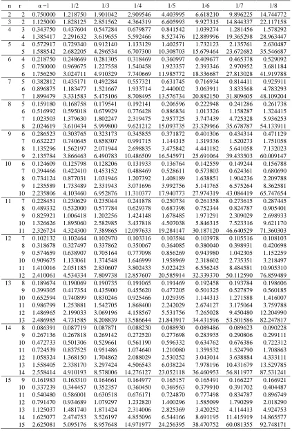
Table 2: Means of spacings of samples of size 2,3,…,15 from the Generalized
Laplace distribution with parameters
1
, and
1, 1 / 2,...,1 / 8
.
n (r, r+1) α =1 1/2 1/3 1/4 1/5 1/6 1/7 1/8
2 (1,2) 1.500000 2.437500 3.802083 5.819092 8.807991 13.236420 19.792450 29.489545 3 (1,2) 1.125000 1.828125 2.851562 4.364319 6.605993 9.927315 14.844337 22.117158 4 (1,2) 1.041667 1.854028 3.072371 4.912589 7.685934 11.850722 18.083841 27.385155 (2,3) 0.687500 0.875208 1.094568 1.359754 1.683085 2.078547 2.562913 3.156584 5 (1,2) 1.015625 1.952865 3.384394 5.574172 8.906132 13.947341 21.536922 32.916200 (2,3) 0.572917 0.729340 0.912140 1.133129 1.402571 1.732123 2.135761 2.630487 6 (1,2) 1.006250 2.055036 3.682771 6.200210 10.062415 15.943341 24.842076 38.238604 (2,3) 0.531250 0.721006 0.946253 1.221989 1.562360 1.983669 2.505574 3.152092 (3,4) 0.437500 0.497338 0.562610 0.636938 0.721994 0.819353 0.930756 1.058184 7 (1,2) 1.002604 2.148106 3.953439 6.774781 11.136731 17.818240 27.976037 43.325910 (2,3) 0.514062 0.748306 1.029384 1.376393 1.808258 2.346977 3.019156 3.857382 (3,4) 0.382812 0.435171 0.492284 0.557321 0.631745 0.716934 0.814411 0.925911 8 (1,2) 1.001116 2.230803 4.197554 7.301736 12.136010 19.582527 30.953459 48.197658 (2,3) 0.506510 0.784612 1.122317 1.543047 2.070891 2.734113 3.567041 4.611838 (3,4) 0.357812 0.426260 0.500389 0.584287 0.680239 0.790379 0.917001 1.062677 (4,5) 0.318359 0.337517 0.359082 0.384283 0.413191 0.445895 0.482571 0.523477
9
Table 3: Means of order statistics of samples of size 2,3,…,15 from the Generalized
Laplace distribution with parameters
1
, and
1, 1 / 2,...,1 / 8
.
n r α =1 1/2 1/3 1/4 1/5 1/6 1/7 1/8
Table 4: Variances of order statistics of samples of size 2,3,…,15 from the Generalized
Laplace distribution with parameters
1
, and
1, 1 / 2,...,1 / 8
.
n r α =1 1/2 1/3 1/4 1/5 1/6 1/7 1/8
2 2 1.4375 0
6.01465 24.0403 6
93.04821 352.56553 1317.8705 3
4884.24640 18005.76893 3 2 1.4149
3
7.27942 32.0987 4
130.7022 5
509.17787 1933.4696 7
7231.34576 26801.02090 4 3 0.5207
2
1.06558 2.20315 4.57972 9.53990 19.89111 41.50265 86.66153 4 1.4417
3
8.49135 39.7040 7
166.7097 1
660.95547 2536.2192 9
9546.20380 35518.32068 5 4 0.5024
6
1.21756 2.81457 6.30610 13.83354 29.91689 64.08329 136.40051 5 1.4702
5
9.54706 46.6356 2
200.5963 3
806.87211 3123.8892 2
11823.9661 4
44147.10548 6 4 0.3033
3
0.45660 0.70769 1.11834 1.78881 2.88444 4.67822 7.62143
5 0.5079 5
1.42476 3.56955 8.40223 19.04224 42.12147 91.69318 197.47816 6 1.4939
5 10.4676 6 52.9883 6 232.6280 5
947.56272 3697.8777 5
14067.5659 3
52693.33247 7 5 0.2912
8
0.49792 0.84998 1.44515 2.44519 4.11971 6.91794 11.58862 6 0.5191
2
1.63551 4.35462 10.64379 24.74683 55.74838 122.99891 267.58271 7 1.5128
2 11.2804 9 58.8611 8 263.0686 2 1083.6472 5 4259.5436 4 16279.8520 6 61162.79536 8 5 0.2103
1
0.26480 0.34724 0.46820 0.64290 0.89400 1.25471 1.77344
6 0.2918 6
0.56966 1.05773 1.90330 3.35305 5.82088 10.00055 17.05425 7 0.5307
3
1.83689 5.13869 12.96203 30.80595 70.52203 157.48408 345.77494 8 1.5278
5 12.0075 1 64.3333 8 292.1337 2 1215.6428 1 4810.0408 8 18463.2829 1 69560.56435 9 6 0.2020
2
0.28052 0.39852 0.57325 0.82972 1.20494 1.75327 2.55450
7 0.2969 4
0.65061 1.29188 2.42928 4.41582 7.84793 13.73109 23.75805 8 0.5412
9
2.02584 5.91046 15.32378 37.13798 86.26316 194.78283 431.34537 9 1.5399
5 12.6652 6 69.4666 8 319.9963 1 1343.9750 0 5350.3400 5 20619.9643 8 77891.05114 1 0
6 0.1595 4
0.17806 0.20869 0.25303 0.31384 0.39553 0.50444 0.64922
7 0.2012 0
0.31363 0.48283 0.73588 1.11223 1.67015 2.49552 3.71491
8 0.3033 7
0.73302 1.53812 2.99996 5.59955 10.15525 18.05491 31.64653 9 0.5504
7
2.20234 6.66555 17.70961 43.68659 102.83605 234.60111 523.69871 1 0 1.5498 4 13.2661 3 74.3092 8 346.7961 3 1468.9967 7 5881.2634 9 22751.7129 1 86158.11897 1 1
7 0.1535 4
0.18523 0.23204 0.29754 0.38690 0.50762 0.67010 0.88854
8 0.2036 9
0.35398 0.58342 0.93175 1.45736 2.24679 3.42816 5.19111
9 0.3098 4
0.81378 1.78978 3.60328 6.88498 12.71569 22.93914 40.69001 1
0
0.5583 6
2.36733 7.40243 20.10710 50.41005 120.13265 276.69369 622.32173 1 1 1.5580 7 13.8195 4 78.8994 1 372.6475 5 1591.0042 6 6403.5152 3 24860.1097 1 94365.17865 1 2
7 0.1278 5
0.13057 0.14093 0.15811 0.18211 0.21371 0.25431 0.30592
8 0.1523 4
0.20318 0.27413 0.37177 0.50491 0.68580 0.93121 1.26398
9 0.2075 2
0.39706 0.69310 1.15095 1.85284 2.92128 4.53865 6.97628
1 0
0.3158 9
0.89164 2.04332 4.23153 8.25837 15.50810 28.35603 50.86058 1
1
0.5651 3
2.52198 8.12090 22.50790 57.27627 138.06462 320.85227 726.76611 1 2 1.5649 9 14.3327 5 83.2678 4 397.6454 1 1710.2488 9 6917.7041 9 26946.5437 0 102515.2654 6 1 3
8 0.1233 2
0.13423 0.15323 0.18045 0.21674 0.26378 0.32408 0.40096
9 0.1535 8
0.22640 0.32658 0.46442 0.65361 0.91287 1.26774 1.75308
1 0
0.2117 6
0.44069 0.80815 1.38816 2.29202 3.68670 5.82220 9.07234
1 1
0.3213 6
0.96620 2.29673 4.87936 9.70893 18.51445 34.28005 62.12937 1
2
0.5709 7
2.66741 8.82136 24.90618 64.25990 156.55850 366.89772 836.63662 1 3 1.5709 0 14.8115 0 87.4397 2 421.8694 3 1826.9464 5 7424.3620 5 29012.2449 7 110611.1001 1 1 4
8 0.1063 0
0.10132 0.10257 0.10837 0.11788 0.13095 0.14776 0.16878
9 0.1220 8
0.14501 0.17714 0.21996 0.27561 0.34721 0.43897 0.55640
1 0
0.1559 9
0.25215 0.38535 0.57046 0.82735 1.18317 1.67507 2.35395
1 1
0.2159 5
0.48381 0.92643 1.63991 2.77026 4.53802 7.27540 11.48161 1
2
0.3262 3
1.03742 2.54883 5.54279 11.22783 21.71889 40.68723 74.46668 1
3
0.5760 3
2.80466 9.50446 27.29781 71.34060 175.55234 414.67441 951.58226 1 4 1.5760 0 15.2603 3 91.4358 8 445.3873 4 1941.2839 5 7923.9569 7 31058.3109 7 118655.1370 6 1 5
9 0.1027 7
0.10331 0.10973 0.12094 0.13654 0.15673 0.18209 0.21349
1 0
0.1226 6
0.15968 0.20799 0.27070 0.35161 0.45580 0.58989 0.76243
1 1
0.1588 8
0.27894 0.44824 0.68712 1.02315 1.49416 2.15222 3.06893
1 2
0.2199 0
0.52589 1.04660 1.90375 3.28392 5.47095 8.89491 14.20534 1
3
0.3305 6
1.10545 2.79889 6.21875 12.80764 25.10731 47.55501 87.84251 1
4
0.5804 6
2.93460 10.1709 8