The McDonald Normal Distribution

On the Occasion of his 75th Birthday Anniversary PJSOR, Vol. 8, No. 3, pages 301-329, July 2012

The McDonald Normal Distribution

Gauss M. Cordeiro Departamento de Estatística

Universidade Federal de Pernambuco gauss@de.ufpe.br

Renato J. Cintra

Departamento de Estatística

Universidade Federal de Pernambuco rjdsc@de.ufpe.br

Leandro C. Rêgo

Departamento de Estatística

Universidade Federal de Pernambuco leandro@de.ufpe.br

Edwin M. M. Ortega

Departamento de Ciências Exatas Universidade de São Paulo edwin@esalq.usp.br

Abstract

A five-parameter distribution called the McDonald normal distribution is defined and studied. The new distribution contains, as special cases, several important distributions discussed in the literature, such as the normal, skew-normal, exponentiated normal, beta normal and Kumaraswamy normal distributions, among others. We obtain its ordinary moments, moment generating function and mean deviations. We also derive the ordinary moments of the order statistics. We use the method of maximum likelihood to fit the new distribution and illustrate its potentiality with three applications to real data.

Keywords: McDonald normal distribution; Maximum likelihood estimation; Mean

deviation; Moment generating function.

1. Introduction

For an arbitrary parent cumulative distribution function (cdf) G x( ), the probability density function (pdf) f x( ) of the new class of McDonald generalized distributions (denoted with the prefix ``Mc'' for short) is defined by

 





1 1

( ) = ( ) ( ) 1 ( ) ,

,

b

ac c

c

f x g x G x G x

B a b



 _{ (1)}

Kumaraswamy (Kw) generalized distributions (Cordeiro & Castro,2010) for a=1. If X

is a random variable with density (1), we write X Mc-G( , , )a b c . The density function (1) will be most tractable when G x( ) and g x( ) have simple analytic expressions. The corresponding cumulative function is

( ) _{1 1}

( ) 0

1

( ) = ( , ) = (1 ) d ,

( , )

c

G x _{a b}

c G x F x I a b

B a b   

 _ 



where 1 1 1

0

( , ) = ( , ) x a (1 ) db x

I a b B a b    _  



Equation (2) can also be rewritten as follows





2 1 ( )

( ) = ,1 ; 1; ( ) ,

( , )

ac

c

G x

F x F a b a G x

aB a b   (3)

where





2 1 , ; ; = ( , ) _{0 (1}(1 )₎ d

b c b

a

t t

F a b c x B b c b t

tz

  

 







function (Gradshteyn & Ryzhik, 2000).

Some mathematical properties of the cdf F x( ) for any Mc-G distribution defined from a parent G x( ) in equation (3), could, in principle, follow from the properties of the hypergeometric function, which are well established in the literature (Gradshteyn & Ryzhik, 2000, Sec. 9.1).

One major benefit of this class is its ability of fitting skewed data that can not be properly fitted by existing distributions. Application of _{X G V}= c( ) _{to a beta random variable V} with positive parameters a and b yields X with cumulative function (2).

The associated hazard rate function (hrf) is





1

( )

( ) ( ) 1 ( )

( ) = .

( , ){1 ( , )}

b

ac c

c G x cg x G x G x x

B a b I a b 



 _



The Mc-G family of densities allows for greater flexibility of its tails and can be widely applied in many areas of engineering and biology.

In this note, we introduce and study the McN distribution for which its density is obtained from (1) by taking G( ) and g( ) to be the cdf and pdf of the normal _{N( , ) }2 distribution. The McN density function becomes

 

1 1

( ) = 1 ,

,

b

ac c

c x x x

f x

B a b

  



   



 _{ }

         _  _{ } 

   

             

where x_, _ is a location parameter,  > 0 is a scale parameter, a, b> 0 and > 0

distribution. Further, the McN distribution with a= 2 and b c= =1 reduces to the skew-normal distribution (Azzalini, 1985) with shape parameter equal to one.

The paper is outlined as follows. Section 2 provides some expansions for the density of the McN distribution. In Section 3, we analyze the bimodality properties of the McN distribution. In Section 4, we derive two simple expansions for its moments. In Sections 5 and 6, we obtain the moment generating function (mgf) and mean deviations, respectively. We derive, in Section 7, an expansion for the density of the order statistics. Section 8 provides two representations for the moments of the order statistics and an explicit expression for the mgf. In Section 9, we derive the hazard rate function and analyze its limiting behavior. In Section 10, the Shannon entropy is derived. Some inferential tools are discussed in Section 11. Applications to three real data sets are illustrated in Section 12. Section 13 ends with some conclusions.

2. Expansion for the Density

Some useful expansions for (1) and (2) can be derived using the concept of exponentiated distributions. Here and henceforth, for an arbitrary parent cdf G x( ), we define a random variable Y having the exponentiated G distribution with parameter a> 0, say

Exp-G( )

Y a , if its cdf and pdf are given by

1

( ) = a( ) and ( ) = ( ) a ( ),

a a

H x G x h x ag x G  x

respectively. The properties of exponentiated distributions have been studied by many authors in recent years. In particular, the exponentiated Weibull (Mudholkar & Srivastava,1995), exponentiated Pareto (R. C. Gupta et al; 1998), exponentiated exponential (R. D. Gupta & Kundu, 2001), and exponentiated gamma (Nadarajah & gupta, 2007) distributions are well documented.

By expanding the binomial in (1), we obtain ( ) 1

=0

1

( ) = ( ) ( 1) ( )

( , )

k k a c

k

b c

f x g x G x

k B a b



  

 

 _{ }

 



and then

( ) =0

( ) = k k a c( ),

k

f x



where h(k a c ) ( )x has the Exp-G[(k a c ) ] distribution and the weights wk are given by

1 ( 1)

= .

( ) ( , )

k

k

b k w

k a B a b

  

 _{ }

  

The Mc-G density function is then a linear combination of exponentiated G densities. The properties of the Mc-G distribution can be obtained by knowing those of the corresponding exponentiated distributions. Integrating (4), we obtain

( ) =0

( ) = k k a c( ).

k

From now on, we work with a random variable Z having the standard McN( , , ,0,1)a b c

distribution. The density of Z reduces to





1

( ) = ( ) ( ) 1 ( ) .

( , )

b

ac c

c

f x x x x

B a b 

 

  

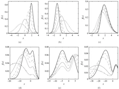
Plots of the McN density for selected parameter values are given in Figure 1. Using (4), we can write

( ) 1

=0

( ) = ( )k a c ( ),

k k

f x



where

 

1 ( 1)

= ( , , ) = .

,

k

k k

b c

k t t a b c

B a b

    _{ }  

We can obtain an expansion for _( )x  _{for  > 0 real non-integer given by}

=0 =0

( ) = j ( 1)j r ( ) .r

j r

j

x x

j r

     

  _{  }

  



We can substitute

 

 

=0

( ) = ( ) ( ) ,r

r r

x   s _ x





where

=

( ) = ( 1)r j .

r

j r

j s

j r

   _    

     



Combining (5) and (6), the McN density function can be expressed as

, =0

( ) = (( ) 1) ( ) ( ).r

k r k r

f x



Figure 1: Plots of the McN(a, b, c, 0, 1) density for some parameter values. (a) a  {0.3, 1, 5, 15, 30}, b = 1, and c = 1, (b) a = 1, b  {0.3, 0.7, 2, 3, 5}, and c = 1, (c) a = 1, b = 0.3, and c  {1, 2, 3, 4, 5}, (d) a  {0.01, 0.03, 0.05, 0.07, 0.09}, b = 0.15, and c = 0.5, (e) a = 0.05, b  {0.02, 0.03, 0.05, 0.07, 0.09}, and c= 0.75, (f) a = 0.01, b = 0.04, and c

 {0.1, 0.2, 0.5, 0.7, 0.9}. In all cases, plots are dotted, solid, dot-dashed, dashed, and bold solid, respectively.

3. Bimodality

The analysis of the critical points of the McN density function furnishes a natural path for characterizing the distribution shape and quantifying the number of modes. Taking the normalization z= x_ , we have

2 2

( ) = ( )[ ( )] [1 ( )]

B( , )

{( 1) ( )[1 ( )] ( 1) ( ) ( ) ( )[1 ( )]}.

ac c b

c c c

f z c _{z z z}

z a b

ac z z c b z z z z z



 

 

 _{  }



          

We refer to the term in curly brackets as s z( ). At the critical points, where f z( ) = 0

z



 ,

we have s z( ) = 0, since the remaining terms of f z( )

z



 are strictly positive. Hence, the

critical points satisfy the following implicit equation

1_{( ) ( )}

= [1 ( 1)] ( ) ( 1) .

1 ( ) ( )[1 ( )]

c

c c

z z

z c a b z a

z z z

   

    

     (8)

By analyzing this expression, the bimodality conditions for the McN density can be established.

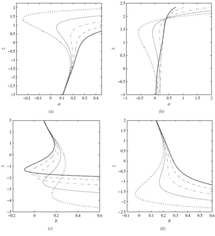
As a particular example, Figure 2(a) gives the plot of the solutions of (8) in terms of a

for a fixed value of b= 0.18. For a= 0.15, there are three solutions indicated by filled dots (). Figure 2(b) provides the corresponding density plots. For a= 0.15, only two of the marked points are indeed modes of the density function, since the remaining point characterizes a local minimum.

Figure 3(a)-(b) give plots of the solutions of (8) in terms of a for a fixed value of c and varying values of b; and for a fixed value of b and varying values of c, respectively. Analogously, Figure 3(c)-(d) provide plots in terms of b. Additionally, we note that the only parts of the implicit curve with probabilistic meaning are those situated in the region

> 0

a and b> 0.

In order to determine which critical points are modes of the distribution, we should consider the sign of the second derivative at the critical points. In particular, a mode of

( )

f z is a critical point with non-positive second derivative. At the critical points, we have

2

2 2

2

( )_{= ( )[ ( )] [1 ( )]} ( )_.

B( , ) ac c b

f z c _{z z z} s z

z a b  z

 

 _{  } 

The sign of 2f z( )₂

z



 is the same of

( )

s z z



 . Then, at a mode, the condition ( ) 0

s z z

 _ 

holds. Explicit evaluation of s z( )

z



 yields

2 1

( ) = ( )[1 c( )] ( ) ( ) ( )c [1 ( 1)] ( ) c ( ).

s z _{z z cz z a a b z c c a b z z}

z  



 _{ }

    _    _    

 (9)

We are now able to prove the following result.

Proposition 1If _c(1 ) = (2 1)(1_b c_{ ac}) _and

2

1

> (2 1)

2

c a

c c

  _{  , then z= 0 is a}

modal point of the McN distribution.

Proof: If s(0) = 0 and s(0) < 0

z



 , then z= 0 is a modal point of the McN distribution.

From the definition of s z( ), it follows that s(0) = 0 if and only if (1 ) = (2 1)(1c )

c b  ac . Letting z= 0 in (9) yields:

1

(0) ₌ 1 ₁ 1 1 1 _{[1 ( 1)].}

2 2c 2 2c

s _{c c a b}

z  

 _  _ _{   }  

  

Using the first order condition _c(1 ) = (2 1)(1 )_b c_{ a and imposing} s(0) < 0 z



 gives

2

1

> (2 1)

2 c

a

c c

  _{  . }

We consider the variational behavior of the critical points of f z( ) with respect to changes in the parameter a. From equation (8), the first derivative of z with respect to

a is

2 1

( )[1 ( )]

= .

( )[1 ( )] ( ) ( ) ( ) [1 ( 1)] ( ) ( )

c

c c c

z c z z

a z z cz z a a b z c c a b z z



  

  

     _    _    

Since _( )[1_{z  }c( )] > 0_{z , the sign of} z

a



 depends entirely on the behavior of the

denominator term. Moreover, except for the sign, this denominator is equal to s z( )

z

  .

Thus, for any z, we have

( )[1 ( )] ( )

= _{( )}c and sign = -sign ,

z c z z z s z

s z

a a z

z



      

   



 _     



where sign( ) _{is the sign function. Further, if} s z( )

z



 is negative at a critical point z, then

z must be a mode which is an increasing function of a. Nevertheless, it is still true that

Proposition 2 2If z is a mode location, then z is an increasing function of a .

We now consider the variational behavior of the critical points of f z( ) with respect to changes in b. From equation (8), the first derivative of z with respect to b is

2 1

( ) ( )

= .

( )[1 ( )] ( ) ( ) ( ) [1 ( 1)] ( ) ( )

c

c c c

z c z z

b z z cz z a a b z c c a b z z



  

 

     _    _    

Since _{c z}( ) ( ) > 0_c _{z , the sign of} z b



 depends entirely on the behavior of the

denominator term. Moreover, this denominator is equal to s z( )

z



 . Thus, for any z, we

have

( ) ( ) ( )

= _{( )}c and sign = sign .

z c z z z s z

s z

b b z

z



     

   



     



Figure 4: (a) c=1, b{0.12,0.16,0.2} _{(solid, dash-dotted, dashed), (b)} c{0.8,1,1.5}

(dotted, solid, dash-dotted).

3.1 Modality Regions

From equation (8), we can express a in terms of z for fixed values of b and c. Let , ( )

b c

a z denote this function of z by fixing b and c. Hence,

, ( ) = 1 _{( )}( ) (1 ₁1/ ) ( ) 1/_{( )} .

c

b c c

z z b c z c

a z

c  z z

 _    

 

Let * ,

b c

Due to its symmetric behavior, the discussion follows mutatis mutandis. So, from equation (8), we can express b in terms of z for fixed values of a and c. Let b za c, ( ) denote such function given by

, 1

1/ [1 ( )]

( ) = 1 1/ .

( ) ( ) ( )

c

a c c c

a c z z

b z a c

z c z  z

 _   _{  }

 

Let * ,

a c

b denote the local maximum of b za c, ( ).

For each implicit curve a zb c, ( ), a critical point could be identified and marked with a bullet. The abscissa values of these critical points indicate the boundary value of a that makes the McN density function switch behavior from a bimodal distribution to a unimodal one. Figure 4(b) shows the modality regions of the McN distribution.

4. Moments

The moments of X having the McN( , , , )a b   distribution are immediately obtained from the moments of Z following the McN( , ,0,1)a b distribution by

=0

( n) = [( ) ] =n n n r r ( )r

r

n

E X E Z E Z

r

 _       



McN distribution. We give two representations for the nth moment of the standard McN distribution, say ' = ( )n

n E Z

 . First, '

n

 can be derived from (5) as

( ) 1

=0

= ( ) ( )d .

' n k a c

n k

k

t x x x x

    

 

 

Setting u= ( ) x , we can write ' n

 in terms of the standard normal quantile function 1

( ) = ( )

Q u _ u _as

1 _{( ) 1}

0 =0

= ( ) d .

' n k a c

n k

k t Q u u u



 

The standard normal quantile function can be expanded as (Steinbrecher, 2002) 2 1

=0

( ) = k ,

k k

Q u



where v= 2 ( u1/ 2) and the bk are calculated recursively from

1

=0

(2 1)(2 2 1)

1

= .

2(2 3) ( 1)(2 1)

k

r k r k

r

r k r b b

b

k r r 



   



Here, b₀ = 1, b₁ = 1/ 6, b₂ = 7 /120, b₃ = 127 / 7560,

By application of an equation in Gradshteyn and Ryzhik (2000, Sec.0.314) for a power series raised to a positive integer, n, we obtain

,

=0 =0

( ) = = .

n

n i i

i n i

i i

Q u _  a v _ c v

Here, the coefficients cn i, for i= 1, 2, are easily obtained from the recurrence equation 1

, 0 ,

=1

= ( ) i [ ( 1) ] ,

n i m n i m

m

c ia  m n i a c 

 



where cn,0 =a0n. The coefficient cn i, can be determined from cn,0, , cn i, 1 and hence from

the quantities a₀, , ai. Equations (12) and (13) are used throughout this article. The

coefficient cn i, can be given explicitly in terms of the coefficients ai, although it is not

necessary for programming numerically our expansions in any algebraic or numerical software.

The coefficients ai in (12) are defined from those in (11) by: ai = 0 for i= 0, 2, 4, and

( 1)/2

=

i i

a b  for i= 1,3,5,, and then the quantities cn i, can be calculated numerically from the ai by (13). We can easily obtain from (10)

/2 ,

, =0 =0

( 1) 2

= (2 ) .

( )

r r i

' i

n k n i

k i r

i r t c

k a c i r

 

 

      

  





The moments of the McN distribution can be determined from equation (14), where the quantities cn i, are derived from (13) using the aiabove.

We now provide a second representation for ' n

 . The standard normal cdf can be expressed as

1

( ) = 1 erf , .

2 2

x

x    x

 _  _{ } 

 

  

The ( , )n r th probability weighted moment (PWM) (for n and r integers) of the standard normal distribution is defined by

, = n ( ) ( )d .r

n r x x x x

  

 



By making use of the binomial expansion and interchanging terms, we have 2

,

=0

1

= erf exp d .

2

2 2 2

r p r

n n r _r

p

r _x x x _x

p





 



      _

     

 

   





Using the series expansion for the error function erf ( )

2 1

=0

2 ( 1)

erf ( ) = ,

(2 1) !

m m

m

x x

m m



  _

we can determine n r, from equations (9)-(11) given by Nadarajah (2008). For n r p  even, we have

/2 ( 1/2) ,

=0 ( )even

( )

1

= 2 2

2 1 1_{; , , ; , , ; 1, , 1 ,}1 3 3

2 2 2 2 2

n r p p

n r

p n r p r p

A

r _{r n r p}

p n r p

F           _    _             _{ }     



where the terms in n r, vanish when n r p  is odd. The moments of the standard McN distribution is calculated from equation (7) as

, , =0

= (( ) 1) ,

'

n k r n r

k r

t s k a c





where_{n r,} is given by (15). Equations (14) and (16) are the main results of this section.

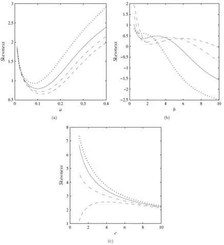
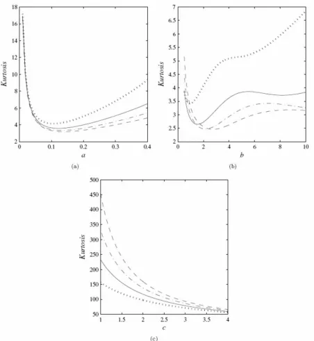
The skewness and kurtosis measures can now be calculated from the ordinary moments using well-known relationships. Plots of the skewness and kurtosis are shown in Figures 5 and 6, respectively. The curves are given for some choices of b as functions of a and

c and for some choices of a as functions of b and c, respectively. These figures immediately reveal that the skewness and kurtosis are very flexible for different values of

a, b, and c.

5. Generating Function

In this section, we provide a representation for the mgf of the McN( , ,0,1)a b distribution, say M s( ) = exp( sZ). From equation (7), we obtain

2

, =0 1

( ) = (( ) 1) ( ) exp d .

2 2 r k r k r x

M s t s k a c x sx x

  _        _  _  





The standard normal cdf ( )x can be expressed as a power series expansion =0

( ) = j

j j x  a x





0 = (1 2 / ) / 2

a _   _,

2 1 = ( 1) 2 2 (2 1) !

j j j a j j    

 for j= 0,1, 2,

and a2j = 0 for j= 1, 2, Thus, we can write

, =0

( ) =r j,

r j j

x c x





where the coefficients cr j_, are calculated from the recurrence equation (13) with ai given

before. We have

2

, , , =0

1

( ) = (( ) 1) exp d .

2 2

j

k r r j

k r j

x

M s t s k a c c x sx x

Figure 5: Skewness of the McN distribution. (a) Function of a for some values of

{0.5,1,1.5, 2}

b (dotted, solid, dot-dashed, dashed) with = 0,  =1 and c=15. (b) Function of b for some values of a{0.5,1,1.5, 2} (dotted, solid, dot-dashed, dashed) with  = 1 _,  =1 and c= 7 (c) Function of c for some values of b{0.5,1,1.5, 2}

Figure 6: Kurtosis of the McN distribution. (a) Function of a for some values of

{0.5,1,1.5, 2}

b _{(dotted, solid, dot-dashed, dashed) with} = 0,  =1 and c=15. (b) Function of b for some values of a{0.5,1,1.5, 2} (dotted, solid, dot-dashed, dashed) with  = 1 ,  =1 and c= 7 (c) Function of c for some values of b{0.5,1,1.5, 2}

By making use of a result by Prudnikov et al. (1986, Eq. 2.3.15.8), the integrals follows as

2 2

( , ) = exp d = ( 1) 2 exp

2 2

j

j j

j

x s

J s j x sx x

s



 

 

_{ }  _    

 

  _{ }  



    



and thus

, , , =0

1

( ) = (( ) 1) ( , ).

2 k r j k r r j

M s t s k a c c J s j









Equation (19) is the main result of this section. The characteristic function (chf)

( ) = [exp(t E itX)]

 of the standard McN distribution is immediately obtained by

( ) = (s M is)

   , where i= 1.

6. Mean Deviations

Let ZMcN( , ,0,1,)a b . The amount of scatter in Z is measured to some extent by the totality of deviations from the mean and median. These are known as the mean deviations about the mean and median, defined by

1( ) =Z ₀ x 1' f x x( )d and 2( ) =Z ₀ x m f x x( )d ,







respectively, where 1' = ( )E Z and m is the median of Z. The measures 1( )Z and 2( )Z

 can be expressed as

1( ) = 2Z 1'F( ) 2 ( ) and1' P 1' 2( ) =Z 1' 2 ( ),P m

        (20)

where

0

( ) = q ( )d

P q



2 1

, , , =0 1

( ) = (( ) 1) exp d ,

2 2

q _j k r j r

k r j

x

P q t c s k a c x x





 

 

  _ _

 





where the coefficients c_{r j,} are obtained from (13) from ai just given before (17).

We can determine ( , ) = exp 2 d

2

q _j x

A j q _x _ _ x

 



2

( 1)/2 0

1

( ) = exp d = 2 .

2 2

j x j j

G j x _  x  _  

  _ _

 



For q< 0,

1

( , ) = ( 1) ( ) ( 1)j j ( , ),

A j q _ G j _{ }  H j q

whereas, for q> 0,

( , ) = ( 1) ( )j ( , ),

where the integral ( , ) = ₀ exp 2 d 2

j j x

H j q x _ _ x

 



Watson, 1990)

2 /4 1/4 /2 1/2

2 /4 1/4, /4 3/4

2 /4 1/4 /2 3/2

2 /4 5/4, /4 3/4

/4 2

( , ) = ( / 2)

( / 2 1/ 2)( 3) /4

2 _{( / 2),}

/ 2 1/ 2

j j q

j j

j j q

j j

q e

H j q M q

j j

q e _{M q}

j              

where M_{k m,} ( )x is the Whittaker function. This function can be expressed in terms of the confluent hypergeometric function

1 1 =0 ( ) ( ; ; ) = ( ) ! k k k k a z F a b z

b k





where ( ) = (a k a a 1) ( a k 1) is the ascending factorial (with the convention that 0

( ) =1a ), by

1/2

, ( ) = exp ₂ m 1 1 1₂ ;1 2 ; .

k m x

M x _ x  F  _{ }m k _ m x

   

   

Hence, we have all quantities to obtain

, , , =0 1

( ) = (( ) 1) ( 1, ),

2 k r j k r j r

P q t c s k a c A j q





  



where A j( 1, )q _{was defined before. Equations (20) and (21) give the mean deviations.}

7. Order statistics

The density function f xi n: ( ) of the ith order statistic for i= 1, , n from data values 1, , n

X  X following the standard McN distribution can be expressed as

1 :

=0 ( )

( ) = ( 1) ( ) .

( , 1)

n i

j i j

i n

j

n i f x

f x F x

j B i n i



  

 

 _{ }

 



We can use the incomplete beta function expansion for  real non-integer

=0 (1 ) ( , ) = , ( , ) ( ) ! m a m x m b x x

I a b

B a b a m m

 _ 



where ( ) = (f _k  f k ) / ( ) f _{. It follows from equations (2) and (6) that}

, =0

(1 ) (( ) )

1

( ) = ( ) ,

( , ) ( ) !

m p p

m p

b s a m c

F x x

B a b a m m

  

 



and then

( ) = ( ) ,p

where

=0

(1 ) (( ) )

1 = ( , ) = . ( , ) ( ) ! m p p p m

b s a m c

v v a b

B a b a m m

  





Thus, the (i j 1)th power of F x( ) can be determined as 1 1 1, =0 =0 ( ) = ( ) = ( ) , i j

i j p p

p i j p

p p

F x v x d x

              





where the coefficients dn p_, are obtained from the recurrence equation

, ,

=1 0 1

= p [ ( 1) ] , = 1,2, ,

n p m n p m

m

d m n p v d p

rv



where dn,0 =v0n. The density function (22) can be rewritten as

: :

, =0

( ) = ( ) ( , ) ( ) ,p r

i n i n

p r

f x  x



where the coefficient g p ri n: ( , ) is given by

: : 1,

=0 =0

1

( , ) = ( , )( , , ) = (( ) 1) ( 1) .

( , 1)

n i j

i n i n k r i j p

k j

n i

g p r g p r a b c t s k a c d

j B i n i

          _{ }  





Equation (23) is the main result of this section. It gives the density function of the McN order statistics as a power series of the standard normal cumulative function multiplied by the standard normal density function.

8. Properties of order statistics

Here, we provide two expansions for the moments and one expansion for the mgf of the McN order statistics. First, the nth moment of the ith order statistic in a sample of size

n, say ( n_: )

i n

E X , of the McN distribution follows from equation (23)

: : ,

, =0

( n ) = ( , ) ,

i n i n n p r p r

E X



where n p r,  is easily obtained from (15). Then, the ordinary moments of the McN order

statistics are simple linear functions of the PWMs of the normal distribution. An alternative formula can be immediately derived from (23) by comparing equations (10) and (14). We have

/2

: : ,

, , =0 =0

( 1) 2

( ) = ( , )(2 ) .

1

j j m

n m

i n i n n m

p r m j

m j

E X g p r c

p r m j

      _{ }      





The mgf of the ith order statistic from the McN distribution, say M si n: ( ), can be written from (23) as

2

: :

, =0 1

( ) = ( , ) ( ) exp d .

2 2

p r

i n i n

p r

x

M s g p r x sx x

Using the same algebraic development of Section 5, we obtain

: : ,

, , =0 1

( ) = ( , ) ( , ),

2

i n i n p r j

p r j

M s g p r c J s j











where J s j( , ) is defined by (18). Equations (24), (25) and (26) are the main results of this section.

9. Hazard Function

The McN hazard rate function takes the form

( )

1 1

1 ( ) =

( , ) 1 _x ( , )

c

ac b

c

x x x

c h x

B a b I _ a b

   _      _    _    _{ }              _{ }  _{ } _{ }           

We study the asymptotic behavior of the hazard function as x . We now show that 2

( ) ( / )

h x  b  x as x . Indeed, we have:

1 1 1 1 1 ( ) =

lim _{( , )} lim lim _{1 ( , )}

( )

1 1

= _{( , )} lim _{1 ( , )} .

( )

b c

ac

x x x

c b c x c x x x

h x c x

x B a b I _x a b

x x

x c

B a b I _x a b

 _       _   _     _                          _{ }          _{ } _   _  _{  }          _{ } _{ }    _

Once again, another indeterminate form arises. An application of L'Hôpital's rule yields 1

2

1 1

lim _{1 ( , )}

( )

1

( )

( , ) 1 1

= _{lim lim} .

1 ( )

b c

x

c

x c x

x x

x

I _x a b

x

B a b b _x x

x

c c x

c  _         _           _{  }          _{ } _{ }    _      _    _       

Another application of L'Hôpital's rule gives

2 1

( )

( , ) 1 1 ₌ ( , ) ₌ ( , )_.

lim lim lim

1 ( )

x c x x

x

B a b b _x x bB a b x bB a b

x

c x c x c

Thus, _{h x( ) ( / ) b }2 _{x as x . It is worth noting that this asymptotic behavior does} not depend on the parameters a c, and . The limit of h x( ) as x  is zero. However, we can verify that

1

( ) ( )

( , )

ac ac

c x x

h x

B a b

 _        _           

 when x .

In fact, considering that

( )

( ) = ( , ) = 0

limx x limx I x  a b



 

  _ 



 , we obtain

1

1 ( ) = 1 .

lim _{( , )} lim

( ) ( )

ac

ac ac ac ac

x x

x

h x c x

B a b

x x x x

       _   _                _{ }       _{ }       _    _      _{ }   _{ }        

Applying L'Hôpital rule, we can show that _{( ) ( ) ( )x  x} 1_{ x . So, we obtain that the} above limit is c/ [B a b( , )].

Rêgo et al. (2012) demonstrated that h x_N( )  x  / 

      

 as x , where h xN( ) is

the normal hazard rate function. Hence, the asymptotic behavior of h x( ) can be related to that one of h xN( ) when x  by





h x h x

B a b

      _      

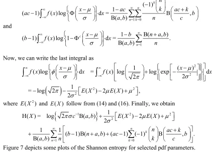
10. Shannon Entropy

Shannon entropy is a measure of uncertainty associated with a random variable. Consider a random variable _{X McN( , , , , )a b c  }2 _{. Thus, the Shannon entropy of X is given by}









H( ) = {log ( ) } = ( )log ( ) d

= ( )log d ( 1) ( )log d

B( , )

( 1) ( )log 1 c d ( )log d .

X E f X f x f X x

c x

f x x ac f x x

a b

x x

b f x x f x x

Figure 7: (a)  = 0,  =1, b{0.1,0.5,1,5,15, 20}, c= 0.75; (b)  = 0,  =1,

{0.1,0.5,1,5,15, 20}

b _, c= 5.

The first integral is simply equal to _log[c1_{B( , )]a b . The second and third integrals can} be expressed in terms of the beta function. Indeed, using Taylor series expansions for the logarithmic function, the previous integrals reduce to

=1 =0

( 1) 1

( 1) ( )log d = B ,

B( , )

k n

n k

n k

x ac ac k

ac f x x b

a b n c

 

 



   _{ }

         

 __{   }

   

 





and

=1

1 B( , )

( 1) ( )log 1 d = .

B( , )

c

n

x b n a b

b f x x

a b n

 

 



     

 _   _{ }

 

 





Now, we can write the last integral as

 

2

2

2 2

2

1 ( )

( )log d = ( ) log log exp d

2 2

1

= log 2 ( ) 2 ( ) ,

2

x x

f x x f x x

E X E X

 



  

  



 

 

   

     _  _  

 

 _ _ _ _ _  _

     

 

  _   _





where _{E X( )}2 _{and E X( ) follow from (14) and (16). Finally, we obtain}





2

=1 =0

1

H( ) = log 2 B( , ) ( ) 2 ( )

2

1 _{1 ( 1)B( , ) ( 1) ( 1) B , .}

B( , )

n k

n k

X c a b E X E X

n ac k

b n a b ac b

k

a b n c

  



 

 

 _   _

     

 _      _{   }

 

 

 





11. Estimation

Here, we determine the maximum likelihood estimates (MLEs) of the parameters of the 2

McN( , , , , )a b c   distribution from complete samples only. Let x1, , xn be a random

sample of size n from this distribution. The log-likelihood function for the vector of parameters _θ= ( , , , , )_{a b c  } T _{reduces to}













=1 =1

=1

( ) = log( ) log ( , ) log ( ) ( 1) log ( )

( 1) log 1 ( ) ,

n n i i i i n c i i

l n c n B a b z ac z

b z           _   _







where = i

i x

z _. The components of the score vector U( )θ are given by













=1 =1 =1

( ) = ( ) ( ) log ( ) ,

( ) = ( ) ( ) log 1 ( ) ,

( )log ( )

( ) = log ( ) ( 1) ,

1 ( )

( )

1 1 ( 1)

( ) = ( ) n a i i n c b i i c n n i i

c i c

i i i

n n

i i

i i i i

U n a a b c z

U n a a b z

z z

n

U a z b

c z

z

ac b c

U z z             _   _       _   _ _   _             













=1 =1 =1

( ) _{( ) ,}

1 ( )

( ) ( ) ( )

1 1 ( 1)

( ) = ,

( ) 1 ( )

c n i i c i c

n n n

i i i i i

i c

i i i i i

z z

z

z z z z z

ac b c

U z z z                    









where_(0)_{( ) is the digamma function. Setting these expressions to zero and solving them} simultaneously yields the MLEs of the five parameters. For interval estimation on the model parameters, we require the expected information matrix. The elements of the 5 5

unit observed information matrix ( )θ are given in Appendix A. Under conditions that are fulfilled for parameters in the interior of the parameter space but not on the boundary, the asymptotic distribution of

 1

5

( ) is (0, ( ) ),

n _{θ θ} N K _θ 

where K( ) = { ( )}θ E  θ is the expected information matrix.

The multivariate normal 1

5(0, ( ) )

N _{ θ}  _{distribution can be used to construct approximate}

confidence intervals and confidence regions for the individual parameters.

given data set. In any case, hypothesis tests of the type _0: = ₀ versus _1:  ₀, where



1: 0 is not true

  is equivalent to compare the McN distribution with the normal distribution and the LR statistic reduces to

    

= 2{ ( , , , , ) (1,1,1, , )},

w _ a b c    _  

where a, b, c, , and  are the MLEs under  and  and  are the estimates under 0

.

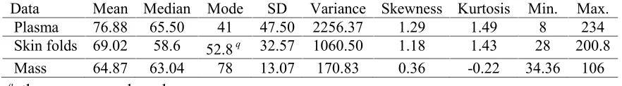
Table 1: Descriptive statistics

Data Mean Median Mode SD Variance Skewness Kurtosis Min. Max.

Plasma 76.88 65.50 41 47.50 2256.37 1.29 1.49 8 234

Skin folds 69.02 58.6 _52.8q _{32.57 1060.50 1.18 1.43 28 200.8}

Mass 64.87 63.04 78 13.07 170.83 0.36 -0.22 34.36 106

q _{there are several modes.}

12. Applications

In this section, we use three real data sets to compare the fits of a McN distribution with some of its sub-models, i.e., the BN, KwN, EN, normal and skew-normal distributions. In each case, the parameters are estimated by maximum likelihood (Section 11) using the SAS subroutine NLMixed. Convergence was achieved using the re-parametrization

=

a ac_.

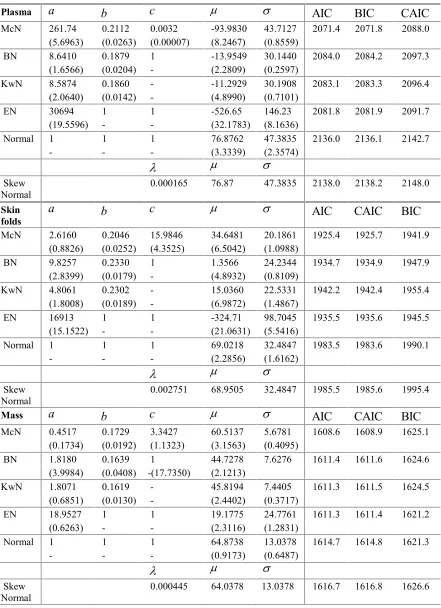
First, we describe the data sets. Then, we report the MLEs (and the corresponding standard errors in parentheses) of the parameters and the values of the AIC (Akaike Information Criterion), CAIC (Consistent Akaike Information Criterion) and BIC (Bayesian Information Criterion) statistics. The lower the values of these criteria, the better the fit. Next, we perform LR tests for the need of skewness parameters. Finally, histograms of the data sets are provided to obtain a visual comparison of the fitted density functions.

Consider the data set discussed in in Weisberg (2005, Section 6.4) which represents 102 male and 100 female athletes collected at the Australian Institute of Sport, courtesy of Richard Telford and Ross Cunningham. The following variables are evaluated in this study:

1. Plasma ferritin concentration (plasma); 2. Sum of skin folds (skin folds);

3. Lean body mass (mass).

We now compute the MLEs and the AIC, BIC and CAIC statistics for each data set. For the three data sets, we fit the McN distribution, with parameters a, b, c,  and  , and this is compared with the fits obtained using the BN, KwN, EN, normal and skew normal distributions. The estimates of  and  for the normal distribution were adopted as initial values.

The results are reported in Table 2. Notice that the three information criteria agree on the model ranking in every case. For the plasma, skin folds, and mass data, the lowest values of the information criteria are obtained from the fit of the McN distribution. Clearly, the McN model having three skewness parameters is preferred for the three data sets.

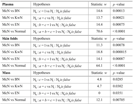
A formal test for the need of the third skewness parameter in the McN distribution can be based on the LR statistics. An application of such method to the current data sets furnishes the results shown in Table 3. For the plasma, skin folds and mass data, we reject the null hypotheses of all three tests in favor of the McN distribution. The rejection is extremely highly significant for the plasma data, and highly or very highly significant for the skin folds data. This gives clear evidence of the potential need for three skewness parameters when modelling real data.

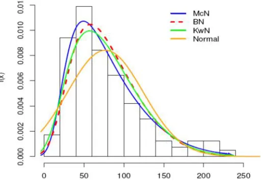
More information is provided by a visual comparison of the histograms of the data with the fitted density functions. The plots of the fitted McN, BN, KwN, normal and skew normal densities are given in Figure 8 for the plasma data, in Figure 9 for the skin folds data, and in Figure 10 for the mass data. In all these cases, the McN distribution provides a closer fit to the histograms than the other four sub-models.

In order to assess whether the model is appropriate, the plots of the estimated survival functions of the McN, BN, KwN and normal distributions and the empirical survival function are given in Figures 11, 12 and 13 for the plasma, skin folds and mass data, respectively. We conclude that the McN distribution provides a good fit for the plasma and skin folds data. For tha mass data, the McN, BN and KwN distributions give reasonable fits, but it is clear that the McN distribution provides a more adequate fit to the histogram of the data.

Table 2: MLEs and information criteria.

Plasma a _b c   _{AIC BIC CAIC}

McN 261.74 0.2112 0.0032 -93.9830 43.7127 2071.4 2071.8 2088.0 (5.6963) (0.0263) (0.00007) (8.2467) (0.8559)

BN 8.6410 0.1879 1 -13.9549 30.1440 2084.0 2084.2 2097.3 (1.6566) (0.0204) - (2.2809) (0.2597)

KwN 8.5874 0.1860 - -11.2929 30.1908 2083.1 2083.3 2096.4 (2.0640) (0.0142) - (4.8990) (0.7101)

EN 30694 1 1 -526.65 146.23 2081.8 2081.9 2091.7 (19.5596) - - (32.1783) (8.1636)

Normal 1 1 1 76.8762 47.3835 2136.0 2136.1 2142.7

- - - (3.3339) (2.3574)

  

Skew

Normal 0.000165 76.87 47.3835 2138.0 2138.2 2148.0 Skin

folds a b c

  _{AIC CAIC BIC}

McN 2.6160 0.2046 15.9846 34.6481 20.1861 1925.4 1925.7 1941.9 (0.8826) (0.0252) (4.3525) (6.5042) (1.0988)

BN 9.8257 0.2330 1 1.3566 24.2344 1934.7 1934.9 1947.9 (2.8399) (0.0179) - (4.8932) (0.8109)

KwN 4.8061 0.2302 - 15.0360 22.5331 1942.2 1942.4 1955.4 (1.8008) (0.0189) - (6.9872) (1.4867)

EN 16913 1 1 -324.71 98.7045 1935.5 1935.6 1945.5 (15.1522) - - (21.0631) (5.5416)

Normal 1 1 1 69.0218 32.4847 1983.5 1983.6 1990.1

- - - (2.2856) (1.6162)

  

Skew

Normal 0.002751 68.9505 32.4847 1985.5 1985.6 1995.4

Mass a _b c   _{AIC CAIC BIC}

McN 0.4517 0.1729 3.3427 60.5137 5.6781 1608.6 1608.9 1625.1 (0.1734) (0.0192) (1.1323) (3.1563) (0.4095)

BN 1.8180 0.1639 1 44.7278 7.6276 1611.4 1611.6 1624.6 (3.9984) (0.0408) -(17.7350) (2.1213)

KwN 1.8071 0.1619 - 45.8194 7.4405 1611.3 1611.5 1624.5 (0.6851) (0.0130) - (2.4402) (0.3717)

EN 18.9527 1 1 19.1775 24.7761 1611.3 1611.4 1621.2 (0.6263) - - (2.3116) (1.2831)

Normal 1 1 1 64.8738 13.0378 1614.7 1614.8 1621.3

- - - (0.9173) (0.6487)

  

Skew

Table 3: LR tests

Plasma Hypotheses Statistic w p-value

McN vs BN ₀: =1c vs 1: 0is false 14.6 0.00013

McN vs KwN ₀: =a cvs 1: 0is false 13.7 0.00021

McN vs EN ₀: = = 1b c vs 1: 0is false 14.4 0.00075

McN vs Normal ₀: = = = 1a b c vs 1: 0is false 70.6 < 0.0001

Skin folds Hypotheses Statistic w p-value

McN vs BN ₀: =1c vs 1: 0is false 11.3 0.00078

McN vs KwN ₀: =a cvs 1: 0is false 18.8 0.000015

McN vs EN ₀: = = 1b c vs 1: 0is false 14.1 0.00087

McN vs Normal ₀: = = = 1a b c vs 1: 0is false 64.1 < 0.0001

Mass Hypotheses Statistic w p-value

McN vs BN ₀: =1c vs 1: 0is false 4.8 0.0285

McN vs KwN ₀: =a cvs 1: 0is false 4.7 0.0302

McN vs EN ₀: = = 1b c vs 1: 0is false 0 0.0351

McN vs Normal ₀: = = = 1a b c vs 1: 0is false 12.1 0.00705

13. Conclusions

A Elements of ( )θ

The elements of the observed information matrix ( )θ for the parameters ( , , , , )a b c  

are

(1) (1) (1)

=1

( ) = [ ( ) ( )], ( ) = ( ), ( ) = n log[ ( )],

aa ab ac i

i

n a  a b n a b z

    



i i i

a a bb

i i i i

z z z

c c _{n b a b}

z z     _{ }         





Figure 9: Fitted McN, BN, KwN, normal and skew normal densities for the skin folds data.

2

2 2

=1

( ){log[ ( )]}

( ) = ( 1) ,

[1 ( )]

c n i i cc c i i z z n _b c z       



( ) 1 ( ) ( ){ log[ ( )] 1}

( ) =

( ) 1 ( )

( ) ( )log[ ( )]

( 1) _,

[1 ( )]

c

n n

i i i i i i

c c

i i i i

c n

i i i i

c

i i

z z z z z c z

a b

z z

z z z z

b c z                      







( ) 1 ( ) ( ){ log[ ( )] 1}

( ) =

( ) 1 ( )

( ) ( )log[ ( )]

( 1) _,

[1 ( )]

c

n n

i i i i i i

c c

i i i i

c n

i i i i

c

i i

z z z z z c z

a b

z z

z z z z

Figure 10: Fitted McN, BN, KwN, normal and skew normal densities for the mass data.

2 2 2

=1

1 1 2 2 2 2

2 2 2

=1 =1

( )[ ( ) ( )]

1 ( ) =

( )

( ) ( ){ ( 1) ( ) ( )} ( ) ( )

( 1) ( 1) _,

1 ( ) [1 ( )]

n

i i i i

i i

c c

n n

i i i i i i i

c c

i i i i

z z z z

n ac

z

z z z c z z z z

b c b c

z z                                







2 2 2 2

=1 =1 =1

2 1 1 2

3 =1

2 2 2

2

3 2 2

=1 =1

( )[ ( ) ( )] ( )

2 1 1

( ) =

( ) ( )

( ) ( )[1 ( 1) ( ) ( )]

( 1)

1 ( )

( ) ( )

( 1) ( 1)

[1 ( )]

n n n

i i i i i i

i

i i i i i

c c

n

i i i i i i

c i i c n n i i c

i i i

z z z z z z

ac ac

z

z z

z z z c z z z

b c

z

z z

b c b c

z                                          













1 ( )

c i i c i z z z    

Figure 12: Estimated survival function by fitting the McN distribution and some other models and the empirical survival for the skin folds data.

Figure 13: Estimated survival function by fitting the McN distribution and some other models and the empirical survival for the skin folds data.

2 2

2 2 2

=1 =1 =1

1 2 1

2 2

=1

1

2

=1 =1

( )[ ( )( 1) ( )] ( )

3 1 1

( ) =

( ) ( )

( ) ( )[1 ( )]{( 1) ( 1) ( )}

( 1)

[1 ( )]

( ) ( )

( 1)

1 (

n n n

i i i i i i i i

i

i i i i i

c c

n

i i i i i i

c

i i

c n n

i i i

c i i

z z z z z z z z

ac ac

z

z z

z z z z z c z

b c

z

z z z

b c



  

  

 

 

 



  

 

  

 

      

 

  

 

 











θ 

, )

i

z

References

1. Azzalini, A. (1985). A class of distributions which includes the normal ones.

Scand. J. Statist,12, 171–178.

2. Cordeiro, G. M., & Castro, M. de. (2010). A new family of generalized distributions.Journal of Statistical Computation and Simulation,81, 883–898. 3. Eugene, N., Lee, C., & Famoye, F. (2002). Beta-normal distribution and its

applications.Communications in Statistics: Theory and Methods,31(4), 497–512. 4. Gradshteyn, I. S., & Ryzhik, I. M. (2000).Table of integrals, series, and products

(6th ed.; A. Jeffrey & D. Zwillinge, Eds.). San Diego: Academic Press.

5. Gupta, R. C., Gupta, R. D., & Gupta, P. L. (1998). Modeling failure time data by Lehman alternatives. Communications in Statistics—Theory and Methods, 27, 887–904.

6. Gupta, R. D., & Kundu, D. (2001). Exponentiated exponential family: an alternative to gamma and Weibull distributions. Biometrical Journal, 43, 117–130.

7. Mudholkar, G. S., & Srivastava, D. K. (1995). The exponentiated Weibull family: a reanalysis of the bus-motor-failure data.Technometrics,37, 436–445.

8. Nadarajah, S. (2008). Explicit expressions for moments of order statistics.

Statistics and Probability Letters,78, 196–205.

9. Nadarajah, S., & Gupta, A. K. (2007). The exponentiated gamma distribution with application to drought data.Calcutta Statistical Association Bulletin,59, 29–54. 10. Prudnikov, A. P., Brychkov, Y. A., & Marichev, O. I. (1986). Integrals and

series: Elementary functions. New York, NY: Gordon & Breach Science Publishers.

11. Rêgo, L. C., Cintra, R. J., & Cordeiro, G. M. (2012). On s