Mixture Distributions and the Construction of Reference Ranges for Biochemical parameters

Reference Ranges for Biochemical parameters

Shahid Kamal Institute of Statistics University of the Punjab Q.A. Campus, Lahore Clive J. Lawrence

Department of Mathematical Statistics & Operational Research University of Exeter, Laver Building

North Park Road, Exeter EX4 4QE, UK Vivian F. Trewin

Department of Pharmacy

Royal Devon and Exeter Hospital (Heavitree) Gladstone Road, Exeter EX1 2ED, UK

Aisha Sekandar Institute of Statistics University of the Punjab Q.A. Campus, Lahore

Abstract

The ability to make use of accurately documented, local and specific, reference ranges is an important part of clinical work. The most readily available, often the only, routinely collected data is that obtained from hospital admissions. A mixture distribution approach is employed to arrive at reference range appropriate to particular groups of patients. A classification rule is used to provide a spectrum of such ranges that allows for the lack of complete separation of the components of the mixture, a common feature when such models are fitted to data. The results of analyses are given for a range of biochemical parameters; in some examples, these are shown separately for males and females, and for those taking, and not taking, a diuretic drug – the most commonly occurring drug-group in the elderly.

1. Introduction

In the course of clinical decision making, reference (sometimes known as ‘normal’, or ‘standard’) ranges are used to assess the significance of the values of biochemical parameters. The use of the term ‘normal’ is somewhat misleading, as has been pointed out by Royston 1_{, in that a value within the range may be}

interpreted to indicate that “individuals falling within such a range are clinically

clinician. Reference ranges of serum electrolytes, creatinine, hemoglobin, and liver enzymes tend to shift to lower values due to the relative shrinkage of organ capacity in the elderly, and so it is often the case that any apparent low values in this age group have no serious implications.

These issues are especially relevant to elderly populations, where the vast majority have at least one clinical condition, varying degrees of change in their body-system functions, and to whom significant drug regimens are commonly administered 2. Shifts in pathological measurements caused by drug treatment will be specific to an individual, and any excessive deviations from drug-related ranges would alert physicians to search for other causes of these abnormal values. The identification of a healthy group of elderly individuals from which to collect information and then construct reference ranges can, for a variety of different reasons, be a difficult, almost impossible task. The most easily available information on the elderly is collected at hospital admission. Although this information will have a number of drawbacks, it does afford the possibility of sufficient case information to be able to construct reference ranges specific to a target group. Where information about a particular biochemical parameter is available for a group of such patients the set of measurements might, at the very least, be thought to have arisen from a mix of both ‘healthy’ and ‘unhealthy’ individuals. This paper considers one way in which this mix might be modeled in order to provide the clinician with an improved tool for his or her assessment.

A considerable body of previous work has addressed various aspects of the construction of reference ranges 1-8. One of the earliest papers, by McPherson et al 3, demonstrated the need for a transformation of the scale of measurement for many biochemical parameters, before any reference range is constructed. Royston et al 1,6,8 in a series of papers have used low-order polynomial curves to produce age-specific ranges, have demonstrated the theoretical and practical advantages of estimating symmetric percentiles of an assumed underlying normal distribution, and have examined the various statistical properties of using the three-parameter log-normal distribution in the calculation of reference ranges for clinical measurements. More recently, Wright and Royston 14 _{have conducted}

a detailed, comparative study of statistical methods used in the determination of age-related reference intervals.

There is also relevant work to be found in other medical research areas where the purpose is to establish some kind of ‘standard’. In the study of human growth, research is often focused upon the estimation of reference centiles of some characteristic of interest (birthweight, birthlength, etc., see for example Lawrence et al 9, Thompson and Theron 10, Cole and Green 11), to provide the clinician with a framework in which to assess the measurement made on a new patient.

any study of this kind a balance needs to be struck between basing the reference values upon known pharmacological effects, the use of data from a very specific group of individuals, where inference to a wider population is not really justified, and the use of a more heterogeneous set of data, such as that from hospital admissions.

2. Method

The population P is assumed to comprise of a mixture of k sub-populations {P1..Pk}. The proportion of each sub-population may or may not be known. Let

c1,..,ck denote these proportions, where ∑ =

k

1 i 1

c and c_i ≥0 for i=1,..,k.The

probability distribution function of a measurement Y in P can be represented in

the mixture form ⎟

⎠ ⎞ ⎜ ⎝ ⎛ = ⎟ ⎠ ⎞ ⎜ ⎝ ⎛ Θ − =

− ∑ i

θ y; F c y; F k 1

i i i , where ⎟⎠

⎞ ⎜ ⎝ ⎛

−i i y;θ

F and ⎟

⎠ ⎞ ⎜ ⎝ ⎛ −i i y;θ

f denote,

respectively. The distribution function and probability density function of Y in Pi,

and, ⎟

⎠ ⎞ ⎜ ⎝ ⎛ ≡ − − − − c;θ;..;θk

Θ denotes the set of unknown parameters to be estimated.

The possible presence of mis-recorded or other unusually high or low values, quite likely for the examples considered in this paper, makes it sensible to assume measurement Y to be ‘censored’ to the interval (L,U). Suppose that in a sample of N measurements, n1 are observed in (L=B0 ≤ Y <B1),.., nM are observed in (BM-1≤Y<BM=U), where ∑

=

= M

1 m m

n

N . Then Prob{Y≤y} = D(y,L)/D(U,L),

where D(a,b) Kc F (a;θ ) F (b;θ ),

1

k∑= k k −k k −k ⎥⎦

⎤ ⎢⎣

⎡ ₋

= and Prob{Bm-1≤Y<Bm}=D(Bm,Bm-1)/D(U, L)=Gm,say. The log-likelihood function is given by In L=constant

+ M n

[

].

m

m − −

=

∑

numerical optimisation techniques, to obtain the ML estimator

−

Θˆ of

−

Θ. Estimates

of the variances (and covariances) of the estimator

−

Θˆ _{can be obtained from the}

matrix . ,

Θ L In . Θ L In E 1 s r − ⎥ ⎥ ⎦ ⎤ ⎢ ⎢ ⎣ ⎡ ⎭ ⎬ ⎫ ⎩ ⎨ ⎧ ∂ ∂ ∂ ∂

where since 0

Θ L In E r = ⎭ ⎬ ⎫ ⎩ ⎨ ⎧ ∂ ∂

for all r, it can be shown that

. Θ G Θ G G N . Θ L In . Θ L In E s m r m M 1 m m s r ∂ ∂ ∂ ∂ = ⎭ ⎬ ⎫ ⎩ ⎨ ⎧ ∂ ∂ ∂ ∂ ∑ =

Assign population element ‘y’ to PA(p) if the estimated conditional probability

{

}

j j j c (y) f c (y) f y Y P ε element Prob ˆ ˆ ˆ ˆ

is ≥ p for some threshold value 0 ≤ p ≤ 1;

otherwise, assign to PR(p). In this paper sub-population Pj was chosen to be the

largest estimated component of the mixture distribution. In all our analyses, this has proved pharmacologically satisfactory. At the lower end of the scale ‘p’ PA(0)

will comprise the original population, and as ‘p’ increases the rule successively restricts PA(p). The nature of the subsequent change in reference range for

successive ‘p’ provides the clinician with an additional information in the assessment of a new patient value.

This classification rule is based upon the optimum decision rule for a Bayesian classifier with rejection, first introduced by Chow12,13, that assigns each population element to that class with maximum aposteriori probability. To allow the acceptance into PA(p) of population elements ‘closer-to’ PR(p), k≠j, Chow’s

procedure needs to be modified to the form given above. The reason for this being that in general verification systems, of which this is an example, the classes (or sub-populations P1..Pk) may be quite close together. When this

occurs, estimation of certain of the parameters in the mixture model will be, with even quite large sample size N, subject to poor precision. This could give rise to a considerable amount of anomalous allocation if the criterion of the maximum a posterior probability is used.

Having established, for a given value of p, the sub-population PA(p), a

single-component model FA(x;θ)

−

− is then fitted and the reference range R100(1−α)%(p)

estimated for specified significance level 100(1−α)%. These calculations produce a spectrum of reference values for the different values of p. At p=0, PA(0)

comprises all the population elements and is identical to P. As p increases, elements not “close to” Pj are removed. A plot of R100(1−α)%(p) against p provides

both a summary of the particular measurement under study and a visual aid to the clinical interpretation of the significance of a measurement for any new patient.

3. Results

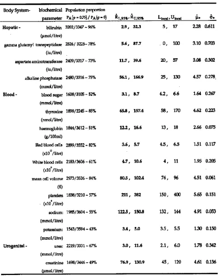
This method of reference range construction is illustrated using hospital admissions data from an Exeter, UK Study 5,7. In each case the mixture model components { ; ⎟}

⎠ ⎞ ⎜ ⎝ ⎛ −i y

95% reference ranges

(

)

(

)

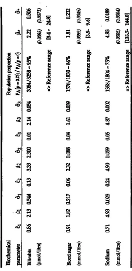
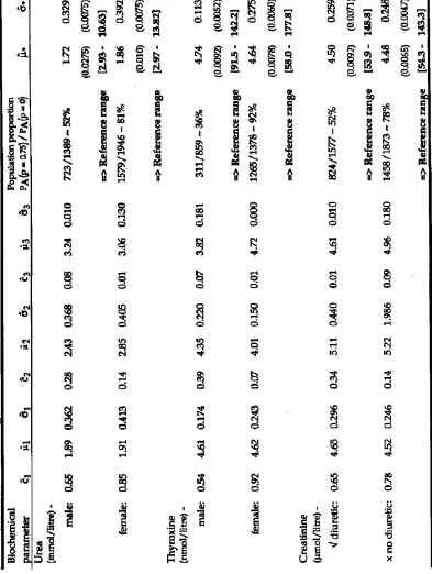
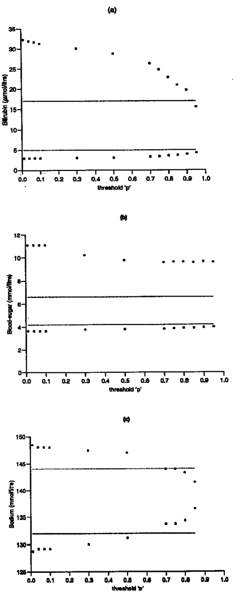
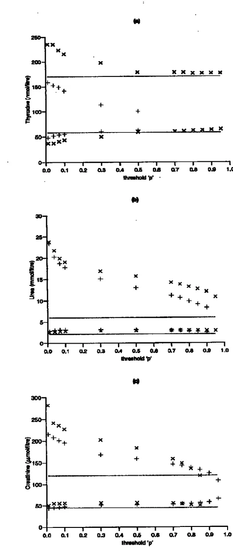
An important objective of reference range determination is to try to produce information for the clinician as relevant as possible to a particular patient group. To illustrate this process summary results from a selection of such analyses are given in Table 2 and the accompanying Figures 1 & 2. Table 2(a) and Figure 1 show the results of analyses applied to a reduced starting population for each of bilirubin, blood-sugar, and serum sodium. In each case, the population was reduced by removing any patient whose drug regimen or disease condition may have affected that particular biochemical parameter. Analyses were carried out for thyroxine and urea to determine separate ranges for males and females, and for creatinine a breakdown into those administered a diuretic drug and those not; the details are given in Table 2(b) and Figure 2.

The results highlight a number of important issues in the construction of reference values. Requiring the estimated conditional probability of belonging to the ‘target’ sub-population to be greater than p=0.75 gives rise to an approximate dichotomy of the set of biochemical parameters. Those which use 70+% of the original population elements (namely, bilirubin, gamma glutamyl transpeptidase, aspartate aminotransferase, alkaline phosphatase, thyroxine, Red blood cells (count), and mean cell volume), and those which use approximately 40-50% (blood-sugar, haemoglobin, White blood cells (count), platelets, sodium, potassium, urea, and creatinine) to establish the reference range. These general reductions are what might be expected with the use of hospital admission data, where the methodology is trying to remove the effects of disease, etc. Another important factor is that the data are from an elderly population (≥ 65 years of age), and will reflect the complicated changes that take place in body-system performance as age increases. Locally-used ranges are often determined from healthy groups of much younger people. For example in Fig 2(b) it is seen that for both males and females, despite some convergence to the locally-used range as we increase ‘p’ and restrict the population on which the range calculation is based, the estimated range remains significantly wider, particularly at the upper limit. In the case of creatinine, Fig 2(c), both the diuretic and non-diuretic groups produce ranges with higher mean values for values of ‘p’ up to 0.85.

resulting in lower values of haemoglobin and Red blood cells, and declining renal function resulting in higher values of creatinine and to some degree urea, with osteoporotic changes accounting for higher values of alkaline phosphatase.

Although the analyses, in Table 2(b), for urea and creatinine, stratified by sex and diuretic-group respectively, indicate certain changes from those reported I Table 1, the ranges are still shifted to higher mean values compared to those of the local ranges. The case of thyroxine is more complicated, since the female group is seen, in Figure 2(a), to ‘validate’ the local range, whilst in the male group many more patient values are rejected, and an estimated range produced which is in agreement at the lower end but with a very significantly reduced upper boundary.

4. Conclusion

We have demonstrated how reference ranges can be determined from observational data that is inevitably going to consist of measurements from a collection of sub-populations in which the individuals are subject to a variety of different influences. For example, factors such as sex, age, and major drug-class regimen must be taken into account in the assessment of unusual or significant clinical measurements. At the same time the methodology needs to be flexible enough to be able to commend itself to simple clinical use, otherwise it will remain a somewhat academic exercise. The use of reference range plots such as we have illustrated enables the clinician to make a more informed interpretation of biochemical results that are presented. The ability to be able to focus attention onto groups of individuals with particular characteristics is important. This requires the availability of large, regularly updated databases, such as hospital-based sets of the kind used in this paper. The obvious disadvantage in using hospital admission data is that the patient set is, by definition, an ill population; although, not uniformly so across all biochemical parameters. However this drawback must be balanced against the need to have sufficient amount of data available, to properly focus the relevance of any reference range, in the way that the methodology in this paper has been able to do.

References

1. Albert, A. and Harris, E. K. (1987). Multivariate Interpretation of clinical Laboratory Data, Marcel Dekker Inc, New York.

2. Chow, C.K. (1957). ‘An optimum character recognition system using decision functions’, IRE Trans. Electronic Computers, 6, 247-254.

3. Chow, C.K. (1970). ‘On optimum recognition error and reject tradeoff’, IEEE Trans. Information Theory, 16 (1), 41-46.

4. Cole, T.J. and Green, P.J. (1992). ‘Smoothing reference centile curves: the LMS method and penalised likelihood’, Statistics in Medicine, 11, 1305-19.

6. Lawrence, C.J. and Trewin, F.V. (1990). “Statistical Methods in the Construction of Pharmacological Reference Ranges and their use in the Identification of Possible Adverse Drug Reactions’. Statistica Applicata, 2(4) 333-349.

7. Lawrence, C.J. and Trewin, F.V. (1991). “the Construction of Biochemical Reference Ranges and the Identification of Possible Adverse Drug Reactions in the Elderly’, Statistics in Medicine, 10, 831-837.

8. Leask, R., Andrews, G. and Caird, F. (1973). ‘Normal values for sixteen blood constituents in the elderly’, Age and Ageing 2, 14-23.

9. Mcpherson, K., Healy, M., Flynn, F., Piper, K. and Garcia-Webb, P. (1978). ‘The effect of age, sex, and other factors on blood chemistry in health’, Clinical Chimica Acta, 84, 373-397.

10. Royston, P. (1991). ‘Constructing time-specific reference ranges’, Statistics in Medicine, 10, 675-690.

11. Royston, P. (1992). “Estimation, Reference Ranges and Goodness-of-fit for the three-parameter log-normal distribution’, Statistics in Medicine, 11, 897-912.

12. Royston, P. and Matthews, J. N. S. (1991). “Estimation of Reference Ranges from Normal Samles’, Statistics in Medicine, 10, 691-695.

13. Thompson, M.L. and Theron G.B. (1990). ‘Maximum Likelihood Estimation of Reference Centiles’, Statistics in Medicine, 9, 539-548.

Table 2a: Maximum Likelihood Estimates for the single-component (with standard errors) and three-component models, in each case natural

Table 2b: Maximum Likelihood Estimates for the single-component (with