A short survey of computational analysis
methods in analysing ChIP-seq data
Hyunmin Kim,1*Jihye Kim,2Heather Selby,2Dexiang Gao,3,4Tiejun Tong,5Tzu Lip Phang6and Aik Choon Tan2,4*
1Department of Biochemistry and Molecular Genetics, University of Colorado School of Medicine, Aurora, CO, USA 2Division of Medical Oncology, University of Colorado School of Medicine, Aurora, CO, USA
3Department of Pediatrics, University of Colorado School of Medicine, Aurora, CO, USA
4Department of Biostatistics and Informatics, University of Colorado School of Public Health, Aurora, CO, USA 5Department of Applied Mathematics, University of Colorado, Boulder, CO, USA
6Division of Critical Care and Pulmonary, Department of Medicine, University of Colorado School of Medicine, Aurora, CO, USA
*Correspondence to:Tel:þ1 303 724 2520; Fax:þ1 303 724 3889; E-mail: [email protected]; E-mail: [email protected]
Date received (in revised form): 9th July 2010
Abstract
Chromatin immunoprecipitation followed by massively parallel next-generation sequencing (ChIP-seq) is a valu-able experimental strategy for assaying protein – DNA interaction over the whole genome. Many computational tools have been designed to find the peaks of the signals corresponding to protein binding sites. In this paper, three computational methods, ChIP-seq processing pipeline (spp), PeakSeq and CisGenome, used in ChIP-seq data analysis are reviewed. There is also a comparison of how they agree and disagree on finding peaks using the publically available Signal Transducers and Activators of Transcription protein 1 (STAT1) and RNA polymerase II (PolII) datasets with corresponding negative controls.
Keywords:CHIP-Seq analysis, Next-generation sequencing, comparative analysis, bioinformatics
Background
The regulation of gene expression is tightly con-trolled by transcription factors (TFs) that bind to specific DNA regulatory regions, histone modifi-cations and positioned nucleosomes in the genome. High-throughput chromatin immunoprecipitation (ChIP) followed by massively parallel next-generation sequencing (ChIP-seq) represents a current approach in profiling genome-wide protein – DNA interactions, histone modifications and nucleosome positions. This new technology has marked advantages over microarray-based (ChIP-chip) approaches by offering higher speci-ficity, sensitivity and coverage for locating TF occu-pancy or epigenetic markers across the genome. ChIP-seq experiments generate large amounts of data (in the order of tens of millions of reads), thus creating a bottleneck for data analysis and
interpretation. Consequently, effective bioinfor-matics tools are needed to process, analyse and interpret these data in order to uncover underlying biological regulatory mechanisms.
In essence, the ChIP-seq analysis workflow can be divided into the following steps:
(i) Pre-processing. The goal of this step is to filter out erroneous and low-quality reads and to ensure that only the highest quality sequencing reads are retained for the sub-sequent mapping step;
on the volume and complexity of target genome sequences. The user can increase specificity using unique reads only or can increase sensi-tivity allowing multiple alignments of reads; (iii) Peak finding. This is the most challenging
step in the analysis workflow, as the goal is to identify significant peak signals among back-ground signals. This includes not only finding the strong signals, but also finding the statisti-cally reproducible weak signals obtained from the modest read counts. To achieve this goal, statistical tests should be based on biologically meaningful background assumptions.
Types of peaks
Peaks in the ChIP-seq data can be classified into three groups: punctate signals (100 base pairs [bp]); localised but broader signals ( kilobase [kb]) and broad signals (100 kb).1 The predictive power of the existing tools depends on the type of data. A mixture of punctate and broader signals is a typical pattern of RNA polymerase II, which occupies tran-scription start sites and promoter – proximal pause sites in a punctate fashion, but the signals diffuse over the body of the transcribed genes.2,3Most algorithms have been optimised to handle the punctate data but are not as good at detecting mixed binding patterns that require non-default parameter settings.
In this paper, three commonly used ChIP-seq computational tools are reviewed in detail, with special emphasis on their underlying peak-calling methods. Information is also provided on the fol-lowing issues: (i) how ChIP-seq methods agree or disagree on different types of data; (ii) the benefits of using the combined methods by comparing these methods on two public datasets.
ChIP-seq processing pipeline (spp)
Spp4was developed as an analysis pipeline specifically designed to detect protein-binding positions with high accuracy by introducing methods to improve tag alignment and to correct for background signals. Spp implemented three peak-calling methods: (i) the window tag density (WTD), which is similar to
XSET5, is a method that extends positive- and negative-strand tags by the expected DNA fragment length in order to determine binding positions to those tags with the highest number of overlapping fragments, and scores positions based on the strand-specific tags; (ii) the matching strand peaks (MSP) approach (which determines local peaks of strand-specific tag density and identifies positions sur-rounded by positive- and negative-strand peaks); (iii) the mirror tag correlation (MTC) method (which scans the genome to identify positions exhibiting pronounced positive- and negative-strand tag patterns that mirror each other). All methods employ back-ground subtraction of the control tag density to correct for the uneven background distribution. The
p-value is calculated assuming Poisson density, and candidate binding sites were selected with p-values
,1025. Given the score s calculated by one of the above methods, the corresponding false discovery rate (FDR) can be estimated as the number of binding positions with the score s or higher found in the ChIP dataset, divided by that in the control set.
CisGenome
CisGenome6 was developed specifically as a suite of tools for ChIP data analysis (both ChIP-chip and ChIP-seq data). For the peak calling method, it uses strand-specific tags to refine peak boundaries and filter out low-quality predictions, and uses a con-ditional binomial model for two-sample analysis (it uses a negative binomial for one-sample analysis) to identify peak regions. Windows passing a user-specified FDR cut-off are used to generate predicted binding regions. Detected windows that overlap with each other are merged into one region. (The minimal FDR among the overlapped windows is taken as the FDR of the region.) There are two post-processing options available in CisGenome: boundary refinement and single-strand filtering.
PeakSeq
the features of open chromatin. As such, this method comprises a two-pass strategy to compen-sate for including control signals in the analysis. In brief, the first pass identifies regions or peaks in the ChIP-seq fragment density map which are substan-tially enriched compared with a simulated simple null background model. To construct the density map, it uses both predefined fragment length and extends tags. Once a fragment density map has been built, control tags are sampled with multiple simu-lations from the subdivided segments (1 megabase [Mb]) in length considering mappability (eg the fraction of uniquely alignable bases in that segment) to generate the null background model. In the second pass, it filters out putative binding sites not significantly enriched compared with the normal-ised control by computing precise enrichments and significances. A peak is deemed statistically signifi-cant based on binomial distribution. The FDR is that estimated for these peaks following the Benjamini and Hochberg7 approach. PeakSeq returns a ranked target list sorted by q-value and fold-enrichment values for each binding site.
Design of ChIP experiment
There are two strategies for ChIP-seq experimental design: one-sample and two-sample experiments. In one-sample analysis, only a ChIP sample is sequenced. In two-sample analysis, both a ChIP sample and a control sample are sequenced. One-sample design (without a control) is a cost-effective strategy after careful post-processing, and some experiments have shown good agreement between one-sample and two-sample analyses.6 The uniform control model5 does not hold due to the biases from non-specific fragments, such as random protein– DNA or antibody– DNA interactions, and the existence of sequencing8and mapping2biases or chromatin structure and genome copy number vari-ations.9,10 Therefore, these intrinsic biases necessitate a control or two-sample analysis.
Peak finding procedure
Due to the intrinsic biases described above, most computational tools recommend the use of a
control in the ChIP-seq analysis for identifying sig-nificant and reliable peaks. The pre-processing and mapping procedures are, in general, followed by the peak-calling steps: (i) create a profile; (ii) select candidate sites; (iii) calculate significance (p-value); and (iv) determine cut-off threshold (ie FDR).
Step1: Creating a signal profile
The ChIP profile is obtained by smoothing the tag counts with or without correcting tag-shifting effects (ie the difference in genomic distance between observed tags and the centre of the actual binding positions). This helps in intrapolating unob-served counts due to low mappability or low cover-age, improving summit resolution (tag reshifting) and exclusion of outliers caused by artefacts. In general, a window of a fixed size develops the profile, sliding across the genome and replacing the tag count at each site with the summed value within the window centred at the site. Spp4 and CisGenome6 merge consecutive windows above a threshold value. The alternative is to use non-overlapping windows as in PeakSeq,2 in which the peaked windows adjacent to each other can be aggregated. There are many modified versions. MACs10 uses the sliding windows after shifting the tags. F-seq11 uses kernel density estimation rather than the summed value. QuEST uses the kernel density approach for devel-oping the strand-specific profile.12
Step 2: Selecting candidate sites or calling peaks
Once generating profile each profile unit satisfies a criterion is considered candidate peaks. The cri-terion is an absolute ChIP signal or a relative enrichment to the background. The utility of this rough selection is twofold. The candidate peaks selected at this step are used to estimate a fragment size and a distance of tag shift. The regions not overlapping with the peaks are used for estimating negative control parameters.
of background model is a Poisson distribution,5,10 assuming a uniform effect of the negative control over the genome. Binomial distribution is an alternative model for utilising the non-uniform effects of the negative control after normalising the sampling ratio between the ChIP and the negative control sample in non-binding regions.6,13
Step 4: Determining cut-off threshold
Given the scores of the peaks, selecting a threshold value is a non-trivial problem. When p-values for the designated distribution are available, they can be used to calculate an FDR.5,6,14,15 Some tools do not providep-values; these generally rank the peaks by the peak height or fold enrichment.4,10,12,16,17 These tools instead calculate an empirical FDR by sampling the tags from the control and ChIP data. The FDR in this case is defined as the ratio of the number of peaks called in the control to the number of peaks called in the ChIP data.
The post-processing step considers tag-shifting effects and predicts the fragment sizes of the library. This consideration is important for prediction of the original binding positions. Spp pre-calculates the autocorrelation between positive- and negative-stranded tag counts to estimate a tag shift. CisGenome takes a two-step approach and corrects these effects in the second step. PeakSeq does not provide automatic correction of tag shifting but allows the user to define the fragment lengths.
Some specialised tools have been developed to analyse broad ChIP peak types — such as those associated with histone modifications — utilising a hidden Markov model18 and a clustering algor-ithm19to find significant patterns.
Preparation of ChIP-seq datasets
The publically available ChIP-seq datasets (after ELAND alignment) were used for human RNA polymerase II (PolII) and STAT1, each with match-ing input-DNA controls (http://www.gersteinlab. org/proj/PeakSeq/). Twenty-eight known human interferon-responsive STAT1 binding sites were obtained from the supplementary material of Robertson et al.5 Data for the known binding sites are available through the ORegAnno database (http:// www.oreganno.org) as dataset OREGDS00006.
Spp provides autocorrelation profiles that can be used to correct for tag shift and define a window size. Ninety-five bp and 60 bp tag shifts and 355 bp and 200 bp window sizes were observed for the STAT1 and PolII datasets, respectively. This infor-mation was used to set up the window sizes for PeakSeq and CisGenome with default settings. The MTC scoring scheme was used for the Spp procedure.
Comparative study of SPP,
CisGenome and PeakSeq on STAT1
and PolII
To compare the predictions of the above three methods, analyses were performed for STAT1 ChIP-seq data with a two-sample approach, using a negative control dataset. A total of 2,716, 5,590 and 1,680 peaks were obtained by applying FDR
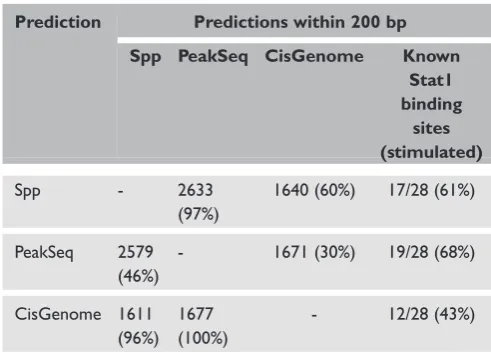
,0.001 to Spp, PeakSeq and CisGenome, respect-ively. Peak median sizes were 190 bp (from the maximum peak of autocorrelations), 450 bp, and 146 bp, respectively. Table 1 summarises the agree-ment between the three peak-finding tools by counting the number of predictions from one tool that overlap within 200 bp of the other tools. Out of 28 known, stimulated STAT1 biding sites, PeakSeq found 68 per cent of them within 200 bp. Table 1. The number of common peaks identified by the three
ChIP-seq analytical tools for Stat1 experimental data
Prediction Predictions within 200 bp
Spp PeakSeq CisGenome Known Stat1 binding
sites (stimulated)
Spp - 2633 (97%)
1640 (60%) 17/28 (61%)
PeakSeq 2579 (46%)
- 1671 (30%) 19/28 (68%)
CisGenome 1611 (96%)
1677 (100%)
Spp and CisGenome found 61 per cent and 43 per cent, respectively. Among the 12 known STAT1 binding sites predicted by CisGenome, 11 and 12 sites overlapped with Spp and PeakSeq predictions, respectively.
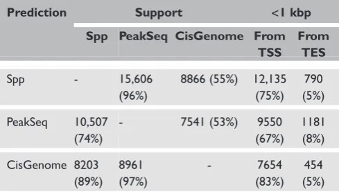
PolII data were also analysed using the same two-sample approach. A total of 16,228, 14,181 and 9,221 peaks were obtained by applying FDR
,0.001, giving median peak sizes of 120 bp, 833 bp and 101 bp using Spp, PeakSeq and CisGenome, respectively. Table 2 summarises the number of common peaks predicted by each method. Based on the genomic coordinates of RefSeq genes (UCSC hg18), it was observed that two-thirds of predicted peaks were within 1 kilo-base pair (kbp) from the transcription start site (TSS), and that peaks were within 1 kbp the tran-scription end sites (TES) to a considerable extent.
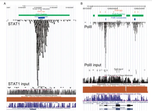
Figure 1 shows examples of peak predictions based on the STAT1 and PolII datasets. The three methods have a good agreement on predicting the centre of STAT1 sites around the known binding sites (black) but Spp (red), PeakSeq (green) and CisGenome (blue) estimated different peak bound-aries due to the different criteria applied at the smoothing and peak-calling steps. For the PolII dataset, only CisGenome specifically predicted peaks at the 50 and 30 ends of the Myc gene. Spp predicted multiple peaks surrounding the 50– 30 boundaries, all of which were included within the clustered peak predictions by PeakSeq over the transcript body. Such inconsistency might have
arisen because these tools were not designed to characterise dynamic PolII patterns.
Discussion and conclusion
Three ChIP-seq computational tools were reviewed in this paper, focusing on their underlying peak-calling methods in particular. These tools were also compared and tested in the analysis of STAT1 and PolII ChIP-seq datasets. From this analysis, it appeared that most of the current ChIP-seq analysis tools were designed for identifying punctuate binding sites. As evident by showing good agree-ment on STAT1 data. By contrast, the predictions for PolII were localised within 1 kbp from the start sites of 70 per cent of RefSeq transcripts. The selected tools were not designed to characterise the trend of PolII occupancy, however, and consistently failed to describe biologically meaningful patterns or secondary peaks observed at the 30 ends in this experimental dataset.
The overall performance of a peak-calling algor-ithm was found to be highly dependent on the smoothing or profiling steps, either by increasing or decreasing the window size. For example, CisGenome with a window size of 100 bp pre-dicted only 900 significant peaks in the STAT1 ChIP-seq experimental data. The tag shifting is another factor that affects performance in some analytical tools. Spp automatically determines this effect, which can be used to specify the fragment extension for PeakSeq and post-correction step in CisGenome.
The quality of ChIP experiments is highly dependent on the enrichment of TF-bound chro-matin compared with background signals. For ChIP-seq analysis, the read number at each chro-mosomal position is related to the number of occu-pied sites in the genome, the range of signal intensity and the bias introduced by sequence pattern and chromatin structure. These parameters are not fully understood in advance and none of the existing ChIP-seq analysis tools can handle all of these possible situations. Integration of genomic contexts such as nucleosome occupancy,20 GC-content8 and multi-species conservation6 will Table 2. The number of common peaks identified by the three
ChIP-seq analytical tools for PolII experimental data
Prediction Support <1 kbp
Spp PeakSeq CisGenome From TSS
From TES
Spp - 15,606 (96%)
8866 (55%) 12,135 (75%)
790 (5%)
PeakSeq 10,507 (74%)
- 7541 (53%) 9550 (67%)
1181 (8%)
CisGenome 8203 (89%)
8961 (97%)
- 7654 (83%)
help to improve prediction performance. The alternative ChIP-chip studies are useful for compar-ing the ChIP-seq results and can help to tune the parameters of methods when it is difficult to find a gold standard test set for PolII.
In summary, ChIP-seq has become an indispensa-ble tool for studying the transcriptional machinery and gene expression regulation on the genome-wide scale. Existing computational software can analyse highly sequence-specific ChIP-seq data with high accuracy. It is likely, however, that new compu-tational methods and more user-friendly workflow will be developed to analyse more complex ChIP-seq data in the future.
Acknowledgments
We would like to thank Dr David L. Bentley for his construc-tive comments on the initial draft of this manuscript. H.K. is supported by NIH grant to GM063873 to D.L. Bentley.
References
1. Pepke, S., Wold, B. and Mortazavi, A. (2009), ‘Computation for ChIP-seq and RNA-ChIP-seq studies’,Nat. MethodsVol. 6 (11 Suppl.), pp. S22–S32. 2. Rozowsky, J., Euskirchen, G., Auerbach, R.K., Zhang, Z.D., Gibson, T.
et al. (2009), ‘PeakSeq enables systematic scoring of ChIP-seq exper-iments relative to controls’,Nat. Biotechnol.Vol. 27, pp. 66 – 75. 3. Baugh, L.R., Demodena, J. and Sternberg, P.W. (2009), ‘RNA Pol II
accumulates at promoters of growth genes during developmental arrest’, ScienceVol. 324, pp. 92 – 94.
4. Kharchenko, P.V., Tolstorukov, M.Y. and Park, P.J. (2008), ‘Design and analysis of ChIP-seq experiments for DNA-binding proteins’, Nat. Biotechnol. Vol. 26, pp. 1351 – 1359.
5. Robertson, G., Hirst, M., Bainbridge, M., Bilenky, M., Zhao, Y.et al. (2007), ‘Genome-wide profiles of STAT1 DNA association using chro-matin immunoprecipitation and massively parallel sequencing’, Nat. MethodsVol. 4, pp. 651 – 657.
6. Ji, H., Jiang, H., Ma, W., Johnson, D.S., Myers, R.M. and Wong, W.H. (2008), ‘An integrated software system for analyzing ChIP-chip and ChIP-seq data’,Nat. Biotechnol. Vol. 26, pp. 1293 – 1300.
7. Benjamini, Y. and Hochberg, Y. (1995), ‘Controlling the false discovery rate: A practical and powerful approach to multiple testing’.J. R. Stat. Soc. Ser. BVol. 57, pp. 289 – 300.
8. Dohm, J.C., Lottaz, C., Borodina, T. and Himmelbauer, H. (2008), ‘Substantial biases in ultra-short read data sets from high-throughput DNA sequencing’,Nucleic Acids Res. Vol. 36, p. e105.
9. Vega, V.B., Cheung, E., Palanisamy, N. and Sung, W.K. (2009), ‘Inherent signals in sequencing-based Chromatin-ImmunoPrecipitation control libraries’,PLoS One, Vol. 4, p. e5241.
10. Zhang, Y., Liu, T., Meyer, C.A., Eeckhoute, J., Johnson, D.S. et al. (2008), ‘Model-based analysis of ChIP-Seq (MACS)’,Genome Biol.Vol. 9, p. R137.
11. Boyle, A.P., Guinney, J., Crawford, G.E. and Furey, T.S. (2008), ‘F-Seq: A feature density estimator for high-throughput sequence tags’, BioinformaticsVol. 24, pp. 2537 – 2538.
12. Valouev, A., Johnson, D.S., Sundquist, A., Medina, C., Anton, E.et al. (2008), ‘Genome-wide analysis of transcription factor binding sites based on ChIP-Seq data’,Nat. MethodsVol. 5, pp. 829 – 834.
13. Xu, H., Handoko, L., Wei, X., Ye, C., Sheng, J.et al. (2010), ‘A signal-noise model for significance analysis of ChIP-seq with negative control’, BioinformaticsVol. 26, pp. 1199 – 1204.
14. Jothi, R., Cuddapah, S., Barski, A., Cui, K. and Zhao, K. (2008), ‘Genome-wide identification of in vivo protein-DNA binding sites from ChIP-Seq data’,Nucleic Acids Res. Vol. 36, pp. 5221 – 5231.
15. Zang, C., Schones, D.E., Zeng, C., Cui, K., Zhao, K. et al. (2009), ‘A clustering approach for identification of enriched domains from histone modification ChIP-Seq data’, Bioinformatics Vol. 25, pp. 1952 – 1958.
16. Johnson, D.S., Mortazavi, A., Myers, R.M. and Wold, B. (2007), ‘Genome-wide mapping of in vivo protein-DNA interactions’, Science Vol. 316, pp. 1497 – 1502.
17. Nix, D.A., Courdy, S.J. and Boucher, K.M. (2008), ‘Empirical methods for controlling false positives and estimating confidence in ChIP-Seq peaks’,BMC BioinformaticsVol. 9, p. 523.
18. Xu, H., Wei, C.L., Lin, F. and Sung, W.K. (2008), ‘An HMM approach to genome-wide identification of differential histone modification sites from ChIP-seq data’,BioinformaticsVol. 24, pp. 2344 – 2349.
19. Hon, G., Ren, B. and Wang, W. (2008), ‘ChromaSig: A probabilistic approach to finding common chromatin signatures in the human genome’.PLoS Comput. Biol. Vol. 4, p. e1000201.