R E S E A R C H
Open Access
MSARC: Multiple sequence alignment by
residue clustering
Michał Modzelewski and Norbert Dojer
*Abstract
Background: Progressive methods offer efficient and reasonably good solutions to the multiple sequence alignment problem. However, resulting alignments are biased by guide-trees, especially for relatively distant sequences.
Results: We propose MSARC, a new graph-clustering based algorithm that aligns sequence sets without guide-trees. Experiments on the BAliBASE dataset show that MSARC achieves alignment quality similar to the best progressive methods.
Furthermore, MSARC outperforms them on sequence sets whose evolutionary distances are difficult to represent by a phylogenetic tree. These datasets are most exposed to the guide-tree bias of alignments.
Availability: MSARC is available at http://bioputer.mimuw.edu.pl/msarc
Keywords: Multiple sequence alignment, Stochastic alignment, Graph partitioning
Background
Determining the alignment of a group of biological sequences is among the most common problems in com-putational biology. The dynamic programming method of pairwise sequence alignment can be readily extended to multiple sequences but requires the computation of ann -dimensional matrix to alignnsequences. Since the size of such a matrix is exponential with respect ton, the time and space complexity of this method is exponential too.
Progressive alignment[1] offers a substantial complexity reduction at the cost of possible loss of the optimal solu-tion. Within this approach, subset alignments are sequen-tially pairwise aligned to build the final multiple align-ment. The order of pairwise alignments is determined by a guide-tree representing the phylogenetic relationships between sequences.
There are two drawbacks of the progressive alignment approach. First, the accuracy of the guide-tree affects the quality of the final alignment. This problem is particu-larly important in the field of phylogeny reconstruction, because multiple alignment acts as a preprocessing step in most prominent methods of inferring a phylogenetic tree of sequences. It has been shown that, within this
*Correspondence: [email protected]
Institute of Informatics, University of Warsaw, Banacha 2, 02-097 Warszawa, Poland
approach, the inferred phylogeny is biased towards the initial guide-tree [2,3].
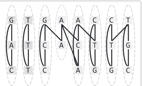
Second, only sequences belonging to currently aligned subsets contribute to their pairwise alignment. Even if a guide-tree reflects correct phylogenetic relationships, these alignments may be inconsistent with remaining sequences and the inconsistencies are propagated to fur-ther steps. To address this problem, in recent programs [4-8] progressive alignment is usually preceded by consis-tency transformation(incorporating information from all pairwise alignments into the objective function) and/or followed byiterative refinementof the multiple alignment of all sequences. Moreover, recently several strategies avoiding guide trees altogether were also proposed [9-11]. In the present paper we propose MSARC, a new non-progressive multiple sequence alignment algorithm. MSARC constructs a graph with all residues from all sequences as nodes and edges weighted with alignment affinities of its adjacent nodes. Columns of best multi-ple alignments tend to form clusters in this graph, so in the next step residues are clustered (see Figure 1). Finally, MSARC refines the multiple alignment corresponding to the clustering.
Experiments on the BAliBASE dataset [12] show that our approach is competitive with the best progres-sive methods and significantly outperforms most non-progressive algorithms. Moreover, MSARC is the best
Figure 1Alignment graph and its desired clustering.Clusters form columns of a corresponding multiple sequence alignment.
aligner for sequence sets with very low levels of conserva-tion. This feature makes MSARC a promising preprocess-ing tool for phylogeny reconstruction pipelines.
Methods
MSARC aligns sequence sets in several steps. In a prepro-cessing step, following Probalign [8],stochastic alignments
are calculated for all pairs of sequences and consistency transformation is applied to resulting posterior probabil-ities of residue correspondences. Transformed probabili-ties, called residue alignment affiniprobabili-ties, represent weights of analignment grapha.
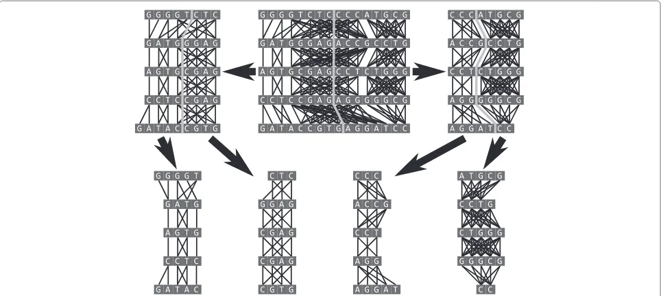
MSARC clusters this graph with a top-down hierarchi-cal method (Figure 2). Division steps are based on the Fiduccia-Mattheyses graph partitioning algorithm [13], adapted to satisfy constraints imposed by the sequence order of residues. Finally, the multiple alignment corre-sponding to the resulting clustering is refined with the iterative improvement strategy proposed in Probcons [7], adapted to remove clustering artefacts.
Pairwise stochastic alignment
The concept of stochastic (or probability) alignment was proposed in [14]. Given a pair of sequences, this frame-work defines statistical weights of their possible align-ments. Based on these weights, for each pair of residues from both sequences, the posterior probability of being aligned may be computed.
A consensus of highly weighted suboptimal alignments was shown to contain pairs with significant probabilities that agree with structural alignments despite the opti-mal alignment deviating significantly. Mückstein et al. [15] suggest the use of the method as a starting point for improved multiple sequence alignment procedures.
The statistical weightW(A)of an alignmentAis the product of the individual weights of (mis-)matches and gaps [16]. It may be obtained from the standard similarity scoring functionS(A)with the following formula:
W(A)=eβS(A), (1)
whereβ corresponds to the inverse of Boltzmann’s con-stant and should be adjusted to the match/mismatch scor-ing functions(x,y)(in fact,β simply rescales the scoring function).
The probability distribution over all alignmentsA∗ is achieved by normalizing this value. The normalization factorZis called thepartition functionof the alignment problem [14], and is defined as
Z=
A∈A∗
W(A)= A∈A∗
eβS(A). (2)
The probabilityP(A)of an alignment can be calculated by
P(A)= W(A)
Z =
eβS(A)
Z . (3)
Let Pai∼bj
denote the posterior probability that residuesaiandbjare aligned.
We can calculate it as the sum of probabilities of all alignments withaiandbjin a common column (denoted byA∗ai∼bj):
Pai∼bj
=
A∈A∗ai∼bj
P(A)= A∈A∗
ai∼bj
eβS(A)
Z
=
Ai−1,j−1
eβS(Ai−1,j−1)
eβs(ai,bj)
⎛ ⎝
Ai+1,j+1
eβS(Ai+1,j+1)
⎞ ⎠
Z
= Zi−1,j−1eβs(ai,bj)Zi+1,j+1
Z .
(4)
Here we use the notation Ai,j for an alignment of the sequence prefixes a1· · ·ai and b1· · ·bj, and Ai,j for an alignment of the sequence suffixesai· · ·amandbj· · ·bn. Analogously,Zi,jis the partition function over the prefix alignments andZi,jis the (reverse) partition function over the suffix alignments.
An efficient algorithm for calculating the partition func-tion can be derived from the Gotoh maximum score algorithm [17] by replacing the maximum operations with additions [14-16]:
ZMi,j =
ZiM−1,j−1+ZiE−1,j−1+ZiF−1,j−1
eβs(ai,bj), (5)
Zi,jE =
Zi,jM−1+Zi,jF−1
eβgo+Zi,jE−1eβgext, (6)
Zi,jF =ZiM−1,j+ZiE−1,jeβgo+ZiF−1,jeβgext, (7)
Figure 2Hierarchical divisive clustering of residues.An alignment graph is recursively partitioned by finding a balanced minimal cut while maintaining the ordering of residues until all parts have at most one residue from each sequence. The final alignment is constructed by concatenating these parts (alignment columns) from left to right.
The reverse partition function can be calculated using the same recursion in reverse, starting from the ends of the aligned sequences.
We also considered a slight modification of formulas 6 and 7:
ZEi,j=ZMi,j−1eβgo+Zi,jE−1eβgext, (9)
ZFi,j=ZMi−1,jeβgo+ZiF−1,jeβgext. (10)
In this case insertions and deletions must be separated by at least one match/mismatch position. This variant was proposed by Miyazawa [14] and applied in the Probalign [8] and MSAProbs [18] aligners.
Alignment graphs
Let us regard probabilitiesPai∼bj
as a representation of a bipartite graph with weighted edges, i.e. a graph with residues from both sequences as nodes and edges joining eachaiwith eachbj.
Given a setSofksequences to be aligned, we would like to analogously represent their residue alignment affinity by ak-partite weighted graph. It may be obtained by join-ing pairwise alignment graphs for all pairs ofS-sequences. However, separate computation of edge weights for each pair of sequences does not exploit information included in the remaining alignments. Thus we decided to address this problem with a so calledconsistency transformation
[4,7], successfully used in progressive methods.
In order to incorporate correspondence with residues from other sequences, MSARC re-estimates the residue alignment affinity according to the following formula:
Pai∼bj
←
c∈S
wacwcb
c∈S
wacwcb
|c|
l=0
P(ai∼cl)P
cl∼bj
,
(11)
wherewxyare weights specifying the relative contribution to the transformation of a sequence pairxy.
If Pab is a matrix of current residue alignment affini-ties for sequences a and b, the matrix form equivalent transformation is given by
Pab←
c∈S
wacwcb
c∈S
wacwcb
Pac·Pcb, (12)
where·stands for matrix multiplication.
MSARC allows for two options of weight assignments. In the first one all the weights are set to 1 and the above formula simplifies to the following:
Pab←
c∈S 1
|S|Pac·Pcb. (13)
In the second option weights are calculated according to the following formula:
wab←
|a|
i=1
|b|
j=1
Pai∼bj
min(|a|,|b|) . (14)
The idea behind the above formula is that the sum of a row/column of a matrix Pab yields the probability that the corresponding residue is aligned to one in the other sequence (not a gap). If sequences a andb are similar, alignments with fewer gaps are preferred, so (at least for the shorter sequence) most of the sums are close to 1. Consequently, thewabis close to 1 as well. On the other hand, weights are much closer to 0 for pairs of dissimilar sequences.
Thus wab measures the similarity of sequences aand
b. Therefore sequences c that are similar to a and b
contribute toPabmore significantly than others.
The consistency transformation may be iterated any number of times, but excessive iterations blur the struc-ture of residue affinity. Following Probalign [8] and Prob-Cons [7], MSARC performs two iterations by default.
Residue clustering
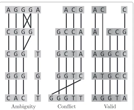
Columns of any multiple alignment form a partition of the set of sequence residues. The main idea of MSARC is to reconstruct the alignment by clustering an alignment graph into columns. The clustering method must satisfy constraints imposed by alignment structure. First, each cluster may contain at most one residue from a single sequence. Second, the set of all clusters must be orderable consistently with sequence orders of their residues. Viola-tion of the first constraint will be calledambiguity, while violation of the second one –conflict(see Figure 3).
Towards this objective, MSARC applies top-down hier-archical clustering (see Figure 2). Within this approach, the alignment graph is recursively split into two parts until no ambiguous cluster is left. Each partition step results from a single cut through all sequences, so clusterings are conflict-free at each step of the procedure. Conse-quently, the final clustering represents a proper multiple alignment.
Optimal clustering is expected to maximize residue alignment affinity within clusters and minimize it between them. Therefore, the partition selection in recursive steps of the clustering procedure should minimize the sum of weights of edges cut by the partition. This is in fact the objective of the well-known problem ofgraph partition-ing, i.e. dividing graph nodes into roughly equal parts such that the sum of weights of edges connecting nodes in different parts is minimized.
The Fiduccia-Mattheyses algorithm [13] is an effi-cient heuristic for the graph partitioning problem. After
Figure 3Clusterings inconsistent (left and middle) and consistent (right) with the alignment structure.
selecting an initial, possibly random partition, it calcu-lates for each node the change in cost caused by moving it between parts, calledgain. Subsequently, single nodes are greedily moved between partitions based on the maxi-mum gain and gains of remaining nodes are updated. The process is repeated in passes, where each node can be moved only once per pass. The best partition found in a pass is chosen as the initial partition for the next pass. The algorithm terminates when a pass fails to improve the par-tition. Grouping single moves into passes helps the algo-rithm to escape local optima, since intermediate partitions in a pass may have negative gains. An additional balance condition is enforced, disallowing movement from a par-tition that contains less than a minimum desired number of nodes.
Fiduccia-Mattheyses algorithm needs to be modified in order to deal with alignment graphs. Mainly, residues are not moved independently; since the graph topology has to be maintained, moving a residue involves moving all the residues positioned between it and a current cut point on its sequence. This modification implies further changes in the design of data structures for gain processing. Next, the sizes of parts in considered partitions cannot differ by more than the maximum cluster size in a final clus-tering, i.e., the number of aligned sequences. This choice implies minimal search space containing partitions con-sistent with all possible multiple alignments. In the initial partition sequences are cut in their midpoints.
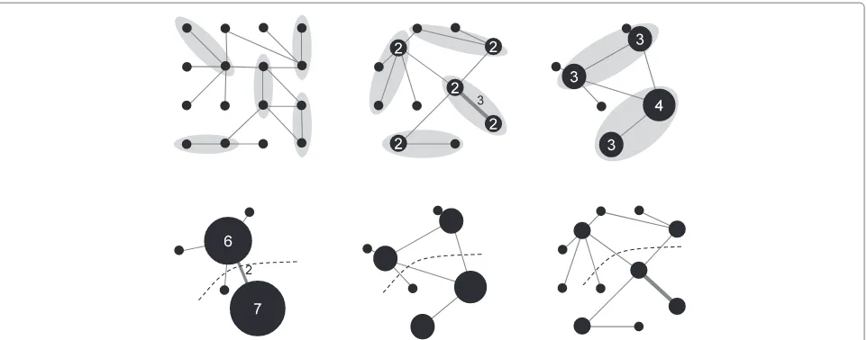
weighted with sums of original weights. The final coars-est graph is partitioned using the Fiduccia-Mattheyses algorithm. Then the partition is projected back to the orig-inal graph through the series ofuncoarsening operations (see Figure 4), each of which is followed by a Fiduccia-Mattheyses based refinement. Because the last refinement is applied to the original graph, the multilevel scheme in fact reduces the problem of selecting an initial partition to the problem of selecting pairs of nodes to be merged. In alignment graphs only neighboring nodes can be merged, so MSARC just merges consecutive pairs of neighboring nodes (see Figure 5).
Refinement
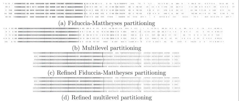
An example of alignment columns produced by residue clustering can be seen in Figure 6(ab). Presented align-ments contain surprisingly many spaces, especially in their right parts. Some of them are clearly superfluous, e.g. in both alignments there are 3 consecutive columns near the right end, each consisting of 4 spaces and 1 G-nucleotide occupying a different row.
Therefore we decided to add a refinement step, follow-ing the method used in ProbCons [7]. Sequences are split into two groups and the groups are pairwise re-aligned. Re-alignment is performed using the Needleman-Wunsch algorithm with the score for each pair of positions defined as the sum of posterior probabilities for all non-gap pairs and zero gap-penalty. First each sequence is re-aligned with the remaining sequences, since such division is very efficient in removing superfluous spaces. Next, several randomly selected sequence subsets are re-aligned against the rest.
Figures 6(cd) show the results of refining the align-ments from Figures 6(ab). Refinement removed superflu-ous spaces from the clustering process and optimized the alignment. Note that the final post-refinement alignments turned out to be the same for both Fiduccia-Mattheyses and multilevel method of graph partitioning.
Löytynoja and Goldman argue in [3] that progressive methods tend to force alignments of non-homologous sequence fragments inserted in corresponding locations of aligned sequences. This tendency leads to systematic errors of the downstream analyses in phylogenetic pipe-lines, including overestimation of substitution and dele-tion events. Unfortunately, iterative refinement may be one of possible source of such effects. Therefore the num-ber of iterations in subset re-alignment step in MSARC is adjustable, in particular the whole step may be turned off.
Computational complexity
Letndenote a number of sequences to align and letlbe their maximum length. Both time and space complexities of stochastic alignment areO(n2l2).
Computations in the other steps use data structures for sparse matrices, so the complexity depends on the
num-ber cof non-zero values per row/column. This number
depends on the cutoff parametertc(entries<tcare set to 0), namelyc≤ 1/tc. However, we observe thatctends to be much lower than this bound, e.g.crarely exceeds 5 for the defaulttc=0.01.
MSARC implementation of consistency transformation requiresO(n2c2l)time. Space complexity of this and the remaining steps is dominated by sparse matrices and equalsO(n2cl).
Figure 5The coarsening of an alignment graph.Lighter colored edges represent edges between the top and bottom sequences, darker edges represent edges between neighboring sequences.
The time complexity of one pass of the Fiduccia-Mattheyses algorithm on whole sequences is O(n2cl2). We observe that the algorithm converges after very few passes, but it is hard to prove a reasonable asymptotic bound. The complexity of the whole clustering is asymp-toticly equal to the complexity of the main partition step.
The time complexity of iterative refinement belongs to the classO(n2cl2).
Results
Benchmark data and methodology
MSARC was tested against the BAliBASE 3.0 benchmark database [1]. It contains manually refined reference pro-tein alignments based on 3D structural superpositions. Each alignment contains core-regions that correspond to the most reliably alignable sections of the alignment. Alignments are divided into five sets designed to evaluate performance on varying types of problems:
RV1X Equidistant sequences with two different levels of conservation
RV11 very divergent sequences (<20%identity)
RV12 medium to divergent sequences (20−40%identity)
RV20 Families aligned with a highly divergent “orphan” sequence
RV30 Subgroups with<25%residue identity between groups
RV40 Sequences with N/C-terminal extensions
RV50 Internal insertions
BAliBASE 3.0 also provides a program comparing given alignments with a reference one. Alignments are scored according to two metrics. A sum-of-pairs score (SP) show-ing the ratio of residue pairs that are correctly aligned, and a total column (TC) score showing the ratio of cor-rectly aligned columns. Both scores can be applied to full sequences or just the core-regions.
We decided to present results based on core-region scores only, since the corresponding sections of the ref-erence alignments are most reliable. Moreover, results for full sequence scores are very similar.
Benchmarking MSARC variants
Two steps of MSARC algorithm: stochastic alignment and iterative refinement follow the respective steps in Probalign [7]. Therefore we decided to set a bunch of related parameters to Probalign’s defaults. Namely, MSARC was run with Gonnet 160 similarity matrix [20], gap penalties of−22, −1 and 0 for gap open, extension and terminal gaps respectively,β=0.2, a cut-off value for posterior probabilities of 0.01 (values smaller than the cut-off are set to 0 and operations designed for sparse matrices are used in order to speed up computations), two itera-tions of the consistency transformation and 100 iteraitera-tions of iterative refinement.
On the other hand, we decided to evaluate three param-eters that seem to be crucial for steps specific for MSARC approach. First, residue clustering may be performed with basic or multilevel Fiduccia-Mattheyses algorithm. Sec-ond, weighted or unweighted consistency transformation may be applied. Third, stochastic pairwise alignment may be based on equations (5)-(8) (i.e. stochastic version of classical Gotoh algorithm) or equations (6) and (7) may be replaced with equations (9) and (10), respectively. The modified formula disallows consecutive insertions and deletions, as is done in Probalign and MSAProbs.
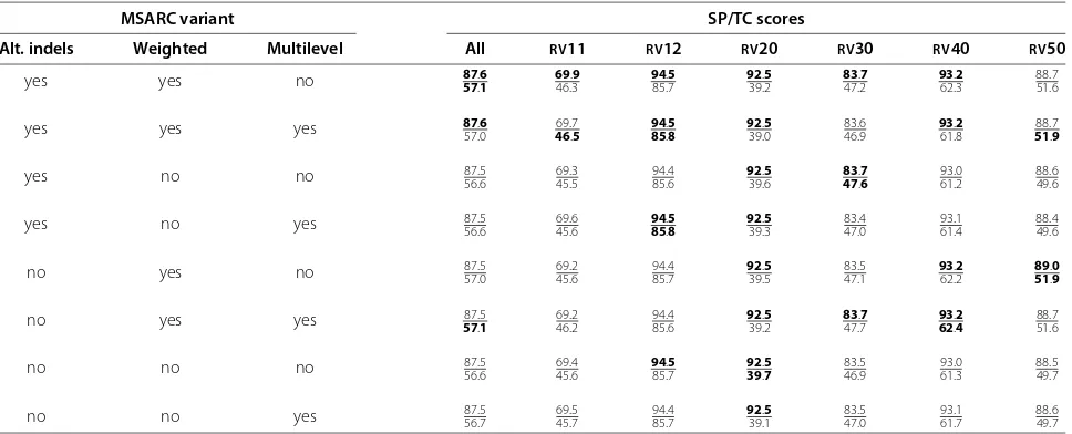
Various combinations of the above options were tested on the BAliBASE sequences. Results are presented in Table 1. The variant with neighboring insertions and
deletions allowed, weighted consistency transformation and residue clustering with basic Fiduccia-Mattheyses algorithm has the best overall results, so it was selected for comparison with other methods. However, the differences are rather marginal.
Comparison to other aligners
MSARC results were compared to CLUSTAL [1,21]
ver. 1.1.0, DIALIGN-T [9] ver. 0.2.2, DIALIGN-TX [22] ver. 1.0.2, MAFFT [6] ver. 6.903, MUSCLE [5] ver. 3.8.31, MSAProbs [18] ver. 0.9.7, Probalign [8] ver. 1.4, ProbCons [7] ver. 1.12, T-Coffee [4] ver. 9.02, FSA [10] ver. 1.15.7 and PicXAA [11] ver. 1.03. All the programs were executed with their default parameters.
Table 2 shows the SP and TC scores obtained by the alignment algorithms on the BAliBASE 3.0 benchmark. The overall results show that MSARC and PicXAA sub-stantially outperform other non-progressive methods –
DIALIGN-T and FSA have SP scores lower by∼10 and
TC scores lower by ∼ 15. Furthermore, MSARC and
PicXAA achieve accuracy similar to the progressive meth-ods MSAProbs and Probalign – the ranges of SP and TC scores of all four programs are 0.2 and 3.6, respectively.
The differences between best programs are not signif-icant in most benchmark series (see Table 3) and corre-spond to their structures – MSARC and PicXAA have the best results for test series RV11 and RV40, and the
worst performance on RV30. Distances in RV30
fami-lies are particularly well represented by guide trees (low similarity between highly conserved subgroups) and pro-gressive methods can benefit from it. On the other hand, seriesRV11 contains highly divergent sequences for which
Table 1 Evaluation of MSARC variants
MSARC variant SP/TC scores
Alt. indels Weighted Multilevel All RV11 RV12 RV20 RV30 RV40 RV50
yes yes no 8757..61 6946.3.9 9485.7.5 9239.2.5 8347.2.7 9362.3.2 88.751.6
yes yes yes 8757.0.6 4669.7.5 8594..58 9239.0.5 46.983.6 9361.8.2 5188.7.9
yes no no 87.5
56.6 45.569.3 94.485.6 9239.6.5 4783..76 93.061.2 88.649.6
yes no yes 87.556.6 69.645.6 8594..58 9239.3.5 83.447.0 93.161.4 88.449.6
no yes no 87.5
57.0 69.245.6 94.485.7 9239.5.5 47.183.5 9362.2.2 8951..09
no yes yes 5787.5.1 69.246.2 94.485.6 9239.2.5 8347.7.7 9362..24 88.751.6
no no no 87.5
56.6 45.669.4 9485.7.5 9239..57 83.546.9 93.061.3 88.549.7
no no yes 87.556.7 69.545.7 94.485.7 9239.1.5 83.547.0 93.161.7 88.649.7
Table 2 Comparison of multiple sequence alignment methods
SP/TC scores Computation
Aligner All RV11 RV12 RV20 RV30 RV40 RV50 BB40037 Time
Non-progressive methods
MSARC 87.6
57.1 6946..93 94.585.7 92.539.2 83.747.2 9362.3.2 88.751.6 9870..70 16 : 36 : 37
DIALIGN-T 77.342.8 49.325.3 88.872.5 86.329.2 74.734.9 82.045.2 80.144.2 52.60.0 1 : 13 : 21
FSA 78.542.1 50.326.9 92.481.8 86.718.7 70.727.6 85.546.2 78.239.8 81.830.0 35 : 15 : 34
PicXAA 8759.4.8 4669.0.3 94.686.2 92.541.6 59.886.0 6293.1.4 89.253.0 9870..70 5 : 54 : 18
Progressive methods
CLUSTAL 84.055.4 59.035.8 90.678.9 90.245.0 86.257.5 90.257.9 86.253.3 61.20.0 12:15
DIALIGN-TX 78.844.3 51.526.5 89.275.2 87.930.5 76.238.5 83.644.8 82.346.6 52.80.0 1 : 36 : 05
MAFFT 86.758.4 65.342.8 93.683.8 92.544.6 85.958.1 91.559.0 90.159.4 56.40.0 54 : 04
MSAProbs 87.8
60.7 68.244.1 9486..65 9246..84 6086..57 92.562.2 9060..88 59.50.0 6 : 43 : 51
MUSCLE 81.947.5 57.231.8 91.580.4 88.935.0 81.440.9 86.545.0 83.545.9 48.40.0 23 : 32
Probalign 87.658.9 69.545.3 9486.2.6 43.992.6 85.356.6 92.260.3 88.754.9 54.20.0 4 : 31 : 41
ProbCons 86.455.8 67.041.7 94.185.5 91.740.6 84.554.4 90.353.2 89.457.3 59.30.0 6 : 56 : 32
T-Coffee 85.755.1 65.540.9 93.984.8 91.440.1 83.749.0 89.254.5 89.458.5 50.90.0 13 : 53 : 02
Columns 2-9 show the mean SP and TC scores for each alignment algorithm on the whole BAliBASE 3.0 dataset, each of its series and caseBB40037. The last column presents total CPU computation time (hh:mm:ss). All scores are multiplied by 100. Best results in each column are shown in bold.
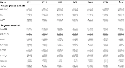
Table 3 Significance of differences in BAliBASE 3.0 SP/TC scores
Aligner RV11 RV12 RV20 RV30 RV40 RV50 Total
Non-progressive methods
DIALIGN-T +8.6e−8
+1.5e−6 ++7.72.2ee−−98 ++1.39.6ee−−75 ++2.70.0024e−6 ++2.14.9ee−−98 ++0.000980.027 ++5.33.6ee−−3626
FSA ++8.61.2ee−−86 ++0.000123.5e−6 ++1.23.6ee−−86 ++2.68.5ee−−66 ++8.31.2ee−−96 ++0.000810.021 ++3.63.5ee−−3427
PicXAA ++(0.0480.53) −−((0.820.98)) −−(0.0550.018) −−7.22.8ee−−56 −+((0.0520.11)) −−((0.0630.37)) −−1.30.0079e−6
Progressive methods
Clustal ++2.65.1ee−−57 ++0.000192.4e−5 −+0.000540.0048 −−0.000600.020 ++2.2(0.16e−)6 −+(0.0170.77) ++1.1(0.30e−13)
DIALIGN-TX +1.0e−7
+1.3e−6 ++4.06.2ee−−87 ++0.000402.3e−7 ++8.70.038e−6 ++2.81.3ee−−97 ++(0.00170.066) ++3.19.5ee−−3423
MAFFT ++0.0031(0.11) ++0.000850.005 −−((0.0520.64)) −−0.00090.0007 ++0.0005(0.07) −−((0.0620.072)) −+(0.0280.55)
MSAProbs ++(0.0280.23) −−((0.670.90)) −−0.000320.011 −−0.000171.4e−5 ++(0.0480.61) −−0.00860.010 −−5.90.020e−8
MUSCLE +7.3e−6
+0.00017 ++0.000152.8e−6 ++0.00015(0.15) + (0.19)
+(0.52) ++7.62.8ee−−96 ++(0.0100.072) ++2.93.3ee−−2212
Probalign ++((0.670.52)) −−((0.880.63)) −−6.80.032e−5 −−0.000560.0099 ++((0.0600.62)) −−((0.320.18)) −−6.00.019e−6
ProbCons ++0.0210.037 ++0.0042(0.19) −+(0.0280.19) −−(0.0100.15) ++0.000260.022 −−((0.120.17)) ++0.00087(0.93)
guide-tree is poorly informative, even if it represents the
correct phylogeny, and RV40 contains sequences with
N/C-terminal extensions which may affect the accuracy of the estimated phylogeny. These sequence families expose progressive methods to guide-tree bias.
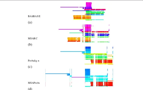
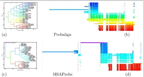
We illustrate this observation with an example of test caseBB40037. As is shown in column 9 of Table 2, MSARC outperforms progressive methods by a large margin. The TC scores of zero means that each alignment method has shifted at least one sequence from its correct posi-tion relative to the other sequences. Figure 7 presents the structure of the reference alignment, as well as alignments generated by MSARC, Probalign and MSAProbs. The large family of red, orange and yellow colored sequences near the bottom has been misaligned by the progressive methods. The reason for this is more visible in Figure 8, where sequences in alignments are reordered according to related guide-trees.
Probalign aligns separately the first half of the sequences (blue and green) and the second half of the sequences (from yellow to red). Next, the prefixes of the second group are aligned with the suffixes of the first group, propagating an error within a yellow sub-alignment.
MSAprobs aligns separately the dark blue, light blue and red sequences. Next the blue sub-alignments are aligned together. The resulting alignment has erroneously inserted gaps near the right ends of dark blue sequences. This error is propagated in the next step, where the suffix of the blue alignment is aligned with the prefix of the red alignment. Finally, the single violet sequence is added to the alignment, splitting it in two.
For both programs, alignment errors introduced in the earlier steps are propagated to the final alignment. On the other hand, the non-progressive strategy used in MSARC yields a reasonable approximation of the reference align-ment (see Figure 7(ab)).
Conclusions
The progressive principle has dominated multiple align-ment algorithms for nearly 20 years. Throughout this time, many groups have dedicated their effort to refine its accuracy to the current state. Other approaches were omitted due to high computational complexity and/or unsatisfactory quality. However, recently several non-progressive methods were proposed. Two of them, PicXAA and MSARC proved to be competitive with the
BAliBAS E
(a)
MSAR C
(b)
Probalig n
(c)
MSAProbs
(d)
Figure 8Guide trees (ac) and alignment visualizations (bd) for test caseBB40037 and programs Probalign (ab) and MSAProbs (cd).Tree branches and aligned sequences are colored based on the evolutionary distances to their neighbors, as computed from the guide-trees used during alignment. Sequences in alignments are ordered following their order in trees, so related sequences have similar color and are positioned together.
best progressive approaches. Moreover, both programs outperform progressive methods on sequence sets with evolutionary distances that are difficult to represent by a phylogenetic tree.
Despite the algorithmic novelty, the non-progressive approaches to multiple alignment are interesting prepro-cessing tools for phylogeny reconstruction pipelines. The objective of these procedures is to infer the structure of a phylogenetic tree from a given sequence set. Multiple alignment is usually the first pipeline step. When align-ment is guided by a tree, the reconstructed phylogeny is biased towards this tree. In order to minimize this effect, some phylogenetic pipelines alternately optimize a tree and an alignment [24-26]. The unbiased alignment pro-cess of MSARC may simplify this procedure and improve the reconstruction accuracy, especially in the most prob-lematic cases.
MSARC has also the potential for quality improve-ments. Alternative methods of computing residue align-ment affinities could be used to improve the accuracy of both MSARC and Probalign based methods. Other approaches to alignment graph partitioning may also lead to improvements in the accuracy of MSARC, for example a better method of pairing residues for multilevel coars-ening than the currently used naive consecutive neighbors merging.
The main disadvantage of MSARC is its computational complexity, especially in the case of the multilevel scheme
variant (MSARC is∼ 2.5× slower than MSAProbs, the
MSARC variant with multilevel scheme is even slower). This is the cost of avoiding the progressive approach.
Endnote
aOur notion of alignment graph slightly differs from
the one of Kececioglu [27]: removing edges between clusters transforms the former into the latter.
Competing interests
The authors declare that they have no competing interests.
Authors’ contributions
ND designed the overall algorithm, participated in its evaluation and wrote the manuscript. MM designed and adapted algorithmic solutions,
implemented the method and participated in its evaluation. Both authors read and approved the final manuscript.
Acknowledgements
This work was supported by the Polish Ministry of Science and Higher Education [N N519 652740].
Received: 1 December 2013 Accepted: 6 April 2014 Published: 16 April 2014
References
1. Thompson JD, Higgins DG, Gibson TJ:Clustal w: improving the sensitivity of progressive multiple sequence alignment through sequence weighting, position-specific gap penalties and weight matrix choice.Nucleic Acids Res1994,22(22):4673–4680.
2. Wong KM, Suchard MA, Huelsenbeck JP:Alignment uncertainty and genomic analysis.Science2008,319(5862):473–476.
3. Löytynoja A, Goldman N:Phylogeny-aware gap placement prevents errors in sequence alignment and evolutionary analysis.Science 2008,320(5883):1632–1635. doi:10.1126/science.1158395.
4. Notredame C, Higgins DG, Heringa J:T-coffee: A novel method for fast and accurate multiple sequence alignment.J Mol Biol2000, 302(1):205–217. doi:10.1006/jmbi.2000.4042.
5. Edgar RC:Muscle: multiple sequence alignment with high accuracy and high throughput.Nucleic Acids Res2004,32(5):1792–1797. doi:10.1093/nar/gkh340.
6. Katoh K, Kuma K-i, Toh H, Miyata T:Mafft version 5 improvement in accuracy of multiple sequence alignment.Nucleic Acids Res2005, 33(2):511–518. doi:10.1093/nar/gki198.
7. Do CB, Mahabhashyam MSP, Brudno M, Batzoglou S:Probcons: Probabilistic consistency-based multiple sequence alignment.
Genome Res2005,15(2):330–340. doi:10.1101/gr.2821705.
8. Roshan U, Livesay DR:Probalign: multiple sequence alignment using partition function posterior probabilities.Bioinformatics,
22(22):2715–2721. doi:10.1093/bioinformatics/btl472.
9. Subramanian AR, Weyer-Menkhoff J, Kaufmann M, Morgenstern B: Dialign-t: an improved algorithm for segment-based multiple sequence alignment.BMC Bioinformatics2005,6:66. doi:10.1186/1471-2105-6-66.
10. Bradley RK, Roberts A, Smoot M, Juvekar S, Do J, Dewey C, Holmes I, Pachter L:Fast statistical alignment.PLoS Comput Biol2009, 5(5):1000392. doi:10.1371/journal.pcbi.1000392.
11. Sahraeian SME, Yoon B-J:Picxaa: greedy probabilistic construction of maximum expected accuracy alignment of multiple sequences.
Nucleic Acids Res2010,38(15):4917–4928. doi:10.1093/nar/gkq255.
12. Thompson JD, Koehl P, Ripp R, Poch O:Balibase 3.0: latest developments of the multiple sequence alignment benchmark.
Proteins2005,61(1):127–136. doi:10.1002/prot.20527.
13. Fiduccia CM, Mattheyses RM:A linear-time heuristic for improving network partitions.InProceedings of the 19th Design Automation
Conference. DAC ’82. Piscataway, NJ, USA: IEEE Press; 1982:175–181.
[http://dl.acm.org/citation.cfm?id=800263.809204]
14. Miyazawa S:A reliable sequence alignment method based on probabilities of residue correspondences.Protein Eng1995, 8(10):999–1009.
15. Mückstein U, Hofacker IL, Stadler PF:Stochastic pairwise alignments.
Bioinformatics2002,18(Suppl 2):153–160.
16. Yu YK, Hwa T:Statistical significance of probabilistic sequence alignment and related local hidden markov models.J Comput Biol 2001,8(3):249–282. doi:10.1089/10665270152530845.
17. Gotoh O:An improved algorithm for matching biological sequences.
J Mol Biol1982,162(3):705–708.
18. Liu Y, Schmidt B, Maskell DL:Msaprobs: multiple sequence alignment based on pair hidden markov models and partition function posterior probabilities.Bioinformatics1964,26(16):1958–1964. doi:10.1093/bioinformatics/btq338.
19. Hendrickson B, Leland R:A multilevel algorithm for partitioning graphs.InProceedings of the 1995 ACM/IEEE Conference on Supercomputing
(CDROM). Supercomputing ’95. New York, NY, USA: ACM; 1995.
doi:10.1145/224170.224228. [http://doi.acm.org/10.1145/224170.224228] 20. Gonnet GH, Cohen MA, Benner SA:Exhaustive matching of the entire
protein sequence database.Science1992,256(5062):1443–1445. 21. Sievers F, Wilm A, Dineen D, Gibson TJ, Karplus K, Li W, Lopez R, McWilliam
H, Remmert M, Söding J, Thompson JD, Higgins DG:Fast, scalable generation of high-quality protein multiple sequence alignments using clustal omega.Mol Syst Biol2011,7:539. doi:10.1038/msb.2011.75. 22. Subramanian AR, Kaufmann M, Morgenstern B:Dialign-tx: greedy and
progressive approaches for segment-based multiple sequence alignment.Alg Mol Biol2008,3:6. doi:10.1186/1748-7188-3-6. 23. Guindon S, Dufayard J-F, Lefort V, Anisimova M, Hordijk W, Gascuel O:
New algorithms and methods to estimate maximum-likelihood phylogenies: assessing the performance of phyml 3.0.Syst Biol2010, 59(3):307–321. doi:10.1093/sysbio/syq010.
24. Redelings BD, Suchard MA:Joint bayesian estimation of alignment and phylogeny.Syst Biol2005,54(3):401–418. doi:10.1080/ 10635150590947041.
25. Lunter G, Miklós I, Drummond A, Jensen JL, Hein J:Bayesian coestimation of phylogeny and sequence alignment.
BMC Bioinformatics2005,6:83. doi:10.1186/1471-2105-6-83.
26. Liu K, Raghavan S, Nelesen S, Linder CR, Warnow T:Rapid and accurate large-scale coestimation of sequence alignments and phylogenetic trees.Science2009,324(5934):1561–1564. doi:10.1126/science.1171243. 27. Kececioglu J:The maximum weight trace problem in multiple
sequence alignment.InProceedings of the 4th Symposium on
Combinatorial Pattern Matching (CPM). Lecture Notes in Computer Science.
Berlin Heidelberg: Springer; 1993:106–119.
doi:10.1186/1748-7188-9-12
Cite this article as:Modzelewski and Dojer:MSARC: Multiple sequence alignment by residue clustering.Algorithms for Molecular Biology20149:12.
Submit your next manuscript to BioMed Central and take full advantage of:
• Convenient online submission
• Thorough peer review
• No space constraints or color figure charges
• Immediate publication on acceptance
• Inclusion in PubMed, CAS, Scopus and Google Scholar
• Research which is freely available for redistribution
![CAMAC bulletin: A publication of the ESONE Committee Issue #14 December 1975 [last pub of series]](data:image/gif;base64,R0lGODlhAQABAIAAAP///wAAACH5BAEAAAAALAAAAAABAAEAAAICRAEAOw==)