R E S E A R C H
Open Access
Recursive algorithms for phylogenetic tree
counting
Alexandra Gavryushkina
1*, David Welch
1and Alexei J Drummond
1,2Abstract
Background: In Bayesian phylogenetic inference we are interested in distributions over a space of trees. The number of trees in a tree space is an important characteristic of the space and is useful for specifying prior distributions. When all samples come from the same time point and no prior information available on divergence times, the tree counting problem is easy. However, when fossil evidence is used in the inference to constrain the tree or data are sampled serially, new tree spaces arise and counting the number of trees is more difficult.
Results: We describe an algorithm that is polynomial in the number of sampled individuals for counting of resolutions of a constraint tree assuming that the number of constraints is fixed. We generalise this algorithm to counting resolutions of a fully ranked constraint tree. We describe a quadratic algorithm for counting the number of possible fully ranked trees onnsampled individuals. We introduce a new type of tree, called a fully ranked tree with sampled ancestors, and describe a cubic time algorithm for counting the number of such trees onnsampled individuals.
Conclusions: These algorithms should be employed for Bayesian Markov chain Monte Carlo inference when fossil data are included or data are serially sampled.
Keywords: Ranked tree, Constraint tree, Resolution, Counting trees, Dynamic algorithms, Bayesian tree prior, Phylogenetics
Background
A phylogenetic tree is the common object of interest in many areas of biological science. The tree represents the ancestral relationships between a group of individuals. Given molecular sequence data sampled from a group of organisms it is possible to infer the historical relation-ships between these organisms using a statistical model of molecular evolution. At present, Bayesian Markov chain Monte Carlo (MCMC) methods are the dominant infer-ential tool for inferring molecular phylogenies [1].
It is a recent trend to include fossil evidence into the inference to obtain absolute estimates of divergence times [2,3]. Fossils may restrict the age of the most resent com-mon ancestor of a subgroup of individuals. This imposes a constraint on the tree topology (the discrete component of a genealogy) and therefore reduces the space of allowable genealogies.
*Correspondence: [email protected]
1Department of Computer Science, The University of Auckland, Auckland, New Zealand
Full list of author information is available at the end of the article
Another trend in phylogenetic analyses is serial (or heterochronous) sampling in which molecular data is obtained from significantly different time points and anal-ysed together. This type of data arises most frequently with ancient DNA and rapidly evolving pathogens [4-6]. In this case tip dates become a part of the genealogy.
Including serially sampled or fossil data modifies or restricts the shape of a phylogenetic tree. Little has been done to describe and classify these modified trees. In this paper, we aim to explore the new spaces formed by these trees.
A genealogy consists of discrete and continuous compo-nents — the tree topology and the divergence times. The tree topologies form a finite tree space when the num-ber of tips is bounded. An important characteristic of this space is the number of trees in it and we aim to find an efficient way to calculate this number.
In the case that fossil data restricts the tree topology, counting the number of trees that satisfy the imposed constraints reveals how much the constraints reduce the tree space.
The number of trees arises as a constant in tree prior distributions. Typically we model the distribution of tree topologies as independent of the distribution of diver-gence times. The density function of the distribution of genealogies is then a product of the density function for the divergence times and the distribution function for tree topologies. A common prior on tree topologies is uniform over all allowable topologies so the distribution function is a constant that is equal to one over the number of tree topologies. When inferring tree topologies using Bayesian MCMC methods, we do not usually need to know this constant but in some cases, as described below, the abso-lute value of the prior distribution is of interest and the constant has to be calculated.
When fossils are used to restrict the age of inter-nal nodes, the tree prior should accurately account for this fact. Heled and Drummond [3] introduced a natu-ral approach for tree prior specification when fossil evi-dence is employed in the inference. Their method requires counting of ranked phylogenetic trees that obey a num-ber of constraints that arise from including the fossil evidence. The construction requires calculation of the marginal density for the time of the calibration node, the node representing the most recent common ancestor of a clade which may or may not be monophyletic. For a particular location of the calibration node, or particu-lar constraints on the tree topology, the marginal density function is the marginal density function for the diver-gence times weighted by the number of trees satisfying the constraints. In this case, the weight constants do not cancel in the MCMC scheme and therefore have to be calculated.
Tree counting has a long history. For phylogenetic trees, the counting problem is to find the number of all possi-ble trees onnleaves. For some types of phylogenetic tree, there are known closed form solutions to this problem. For other types, only recursive equations have been derived. In this paper, we consider only rooted trees.
A survey of results on counting different types of rooted trees is presented in [7] where trees with different com-binations of the following properties are considered: trees are either labeled (only leaves are labeled) or unlabeled, ranked or non-ranked, and bifurcating or multifurcating. The results presented in the survey can also be found in [6,8,9].
In [10], Griffiths considered unlabeled, non-ranked rooted trees such that interior nodes can have one child or more and the root has at least two children. Using generating functions, he derived recursive equations for counting the number of all possible such trees on n leaves withs interior nodes. In [11], Felsenstein consid-ered partially labeled trees, i.e., a tree in which all the leaves are labeled and some interior nodes also may be labeled. He derived the recursive equations for counting
the number of rooted, non-ranked, partially labeled trees withnlabeled nodes.
In this paper, we consider a number of counting prob-lems for different classes of phylogenetic trees. First, we describe an effective way of counting the number of all possible fully ranked trees onnleaves, that is, trees onn leaves in which all internal and leaf nodes are ranked.
Second, we find the number of bifurcating trees that resolve a given multifurcating tree withnleaves. We give a solution to this problem for rooted, ranked, labeled trees and generalise the algorithm to count resolutions to fully ranked trees.
Finally, we introduce and formally describe a new type of phylogenetic tree and describe an algorithm for counting the number of all such trees onnleaves. This type of tree is important when we have a serial sample and sampled individuals can be direct ancestors of later sampled indi-viduals. When the population size is small or the fraction of individuals sampled from the population is large, this type of tree should be included in the inference [12,13].
Serial sampling
We mainly follow the terminology from [9] for the defi-nitions of phylogenetic trees. A tree is a finite connected undirected graph with no cycles. A rooted tree is a tree with a single nodeρ designated as a root. Every rooted treeT = (V,E,ρ)imposes a partial order onV that is defined as follows:v1≤T v2if a unique simple path from the root tov2passes throughv1. So the root is the small-est element. Ifv1≤T v2then we say thatv1is an ancestor ofv2andv2is a descendant ofv1. A node in a rooted tree is called interior if it has descendants and a leaf if it has no descendants. The root is considered interior. Denote
◦
V the set of interior nodes ofT. A nodeuis a parent of a nodevandvis a child ofuif v <T uand there is no
w ∈ V such thatv <T w <T u. A rooted tree is called
binary if every interior node has exactly two children. It is called weakly binary if every interior node has at most two children. We have chosen this terminology to fit with the usage of “binary” in the phylogenetics literature which may not agree with that in other literatures.
setV◦ into the set{1,. . .,|V◦|}such thatv1 ≤T v2implies h(v1)≤h(v2)for everyv1,v2∈
◦
V. In other words, there is a linear order on the interior nodes ofT that is consistent with the partial order ofT.
Definition 1.A ranked X-treeis a binary ranked phy-logenetic X-tree.
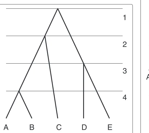
An example of a ranked tree is given in Figure 1. In biology, a phylogenetic tree represents the evolution-ary history of a collection of sampled individuals. The collection of individuals is represented by the setX. The root of the tree is the most recent common ancestor of X and interior nodes are bifurcation events. The rank-ing function represents the time order of the bifurcation events. A general problem in evolutionary biology is how to reconstruct the phylogenetic tree from sequence data obtained from sampled individuals. Tackling this prob-lem in a Bayesian framework may require counting the number of all possible histories on a sample of individuals. When all individuals are sampled at the same time (as in Figure 1) counting tree problem has a simple solution.
LetXbe a fixed label set such that|X| =n. The number of all rankedX-trees up to isomorphism is
R(n)= n!(n−1)! 2n−1
This formula has been derived by many authors. Proofs can be found in [6,7], or [9]. The letterRin the equation comes from the word “ranked”.
A
B
C
D
E
1
2
3
4
Figure 1Ranked tree.RankedX-tree,X= {A,B,C,D,E}. The numbers on the right are values of the ranking function.
The situation is different when individuals are sampled at different times (serially sampled). In this case, we need to define another kind of phylogenetic tree in which leaves are also ranked.
Definition 2.A fully ranked (FR) X-tree is a pair (T,h), whereT is a binary rooted phylogenetic X-tree and h : V → {1,. . .,l}with |V◦| < l ≤ |V| is a surjective function such that
• v1≤Tv2impliesh(v1)≤h(v2)and
• h(v1)=h(v2)impliesv1=v2orv1,v2∈V\ ◦ V.
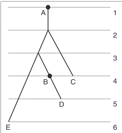
An example of a fully rankedX-tree is given in Figure 2. Before the tree is reconstructed we observe only leaves (sampled individuals) of the tree that are grouped (pre-ranked) according to the times they were sampled. For the tree shown in Figure 2, we have two sampling times and hence two groups:A,B, andCform the first group;Dand Eform the second group.
LetT = (T,h)be a fully rankedX-tree withh : V → {1,. . .,l}. Let m = |h(φ (X))|, that is, the number of sampling times. Define a pre-ranking function hˆ from X onto {1,. . .,m} for tree T such that for all x1,x2∈X
• h(φ (x1))≤h(φ (x2))impliesh(xˆ 1)≤ ˆh(x2)and • h(φ (x1))=h(φ (x2))iffh(xˆ 1)= ˆh(x2).
1
2
3
4
5
6
A
B
C
D
E
For the tree given in Figure 1,h(A)ˆ = ˆh(B) = ˆh(C) = 1 andh(D)ˆ = ˆh(E)=2.
LetXandhˆ : X → {1,. . .,m}be fixed. We are inter-ested in the number of all fully rankedX-trees that havehˆ as a pre-ranking function. Note that this number depends only on the numbersni = |{x|ˆh(x) = i}|, the number of
individuals sampled at theith time point, not onXandhˆ directly. We denote this quantity byF(n1,. . .,nm), where
Fstands for “fully ranked”. Then
F(n1,. . .,nm)= nm
i=1
R(nm)
R(i) F(n1,. . .,nm−1+i) (1)
andF(n)=R(n).
Proof. Consider a continuous process of bifurcation in which lineages may bifurcate in time or be cut and labeled (sampled). The process finishes when all lineages are cut producing a tree. The discrete structure of the tree pro-duced by this process is a fully rankedX-tree. It is easy to see that every fully ranked X-tree can be obtained as a result of this process. To count the required number we can count the number of different trees which can be produced by the process if we know that after it finishes there arenisampled individuals (i.e., cut and labeled
lin-eages) at the ith time point, i.e., we have the sequence (n1,. . .,nm).
Suppose that at the (m − 1)th time point there are i lineages that are ancestral to nm individuals sampled
at time m. When we look at this process backwards in time the bifurcation events become coalescence events. The number of different ways thesenmlineages coalesce
to i lineages is RR(nm(i)). This is the number of all possi-ble ranked X-trees on nm individuals but since we are
not interested in the structure of the coalescent after we reach i lineages, it is divided by the number of ways in which the remaining i lineages can coalesce. Note that if coalescence patterns are different between the (m−1)th and mth time points then the trees are also different.
Further, for each of these coalescence patterns, we need to count the number of different ways theseilineages and other n1,. . .,nm−1 lineages can coalesce. This is where
we can apply the recursion. We can consider that we also cut these i lineages at time m− 1 and label them with the ranked subtrees descendant from these lineages. Then, at time m − 1, we have nm−1 sampled
individ-uals and another i sampled individuals and it remains to count the number of trees on the sequence (n1,. . ., nm−1+i).
Note that two trees are different if they have different numbers of lineages at timem−1. The number of
addi-tionalilineages can be between 1 andnmand we need to
sum over all possibleito complete the recursion.
We introduce a third type of tree in which sampled individuals may be direct ancestors of later sampled indi-viduals. We call it a tree with sampled ancestors. This type of tree is not usually considered in phylogenetics since the probability of sampling a direct ancestor is often negligible. In small populations or when a large portion of the population is sampled, however, this can not be ignored.
LetT =(V,E,ρ)be a weak binary tree. Define a setVˆ as follows:
ˆ
V={v∈V|deg(v)=1 or [deg(v)=2 andvis not the root]}
A rooted S-phylogenetic X-tree is a pair T = (T,φ), where T is a weak binary tree and φ : X → ˆV is a bijection.
Definition 3.A fully ranked X-tree with sampled ancestors (FRS X-tree)is a pair(T,h), whereT is a rooted S-phylogenetic X-tree and h:V → {1,. . .,l}is a surjective function such that
• v1<T v2impliesh(v1) <h(v2)and • h(v1)=h(v2)impliesv1=v2orv1,v2∈ ˆV;
(see Figure 3).
The definition of a pre-ranking function remains the same for FRS trees. Let S(n1,. . .,nm) (with S standing
for ‘sampled ancestors’) denote the number of all FRSX -trees that have the same pre-ranking function hˆ, where ni= |{x| ˆh(x)=i}|. Then
S(n1,. . .,nm)= nm
i=1
min{i,nm−1}
j=0
i j
nm−1
j
×R(nm)
R(i) S(n1,. . .,nm−1+i−j) (2)
andS(n)=R(n).
Proof. Consider the same process as before with only change of sampling events. Now, at some points of time, some lineages are cut and labeled and others are only labeled but not cut.
Then this equation can be obtained as follows. We have nm individuals that are sampled at the mth time point.
At timem−1, there are between 1 andnmancestral
A
B
C
D
E
1
2
3
4
5
6
Figure 3FRS tree.FRSX-tree with the labeled 1-degree root.X= {A,B,C,D,E}. The numbers on the right are values of the ranking function.
of coalescence between timesmandm−1. Letidenote the number of these lineages. Then there are RR(nm(i)) dif-ferent possible coalescent patterns that can lead to this situation. Some of theseiancestral lineages may be among the individuals sampled at timem−1, i.e. lineages that are labeled but not cut at timem−1. Letjbe the num-ber of those ancestral lineages that are sampled at time m−1. There areijways to chose these jlineages out of i and there are nm−1
j
possible ways to chosej sam-pled at timem−1 individuals that are not cut at time m−1.
Further, at timem−1, there arenm−1sampled lineages andi−j ancestral lineages that are not sampled and it remains to count the number of FRS trees on the sequence (n1,. . .,nm−1+i−j).
Finally, we sum over all possibleiandjto complete the recursion.
Dynamic counting
Calculating the recursions (1) and (2) directly is ineffi-cient and impractical. Here we describe a more effiineffi-cient algorithm for counting fully ranked trees using these recursions. Rewrite equation (1) as
F(n1,. . .,nm)=R(nm) nm
i=1
F(n1,. . .,nm−1+i) R(i)
Then instead of calculating F(n1,. . .,nj +α) forj ∈
{1,. . .,m−1}andα ∈ {0,. . .,nj+1+. . .+nm}we can
calculate
Aj(α)= F(n1,. . .,nj+α)
R(α) (3)
using recurrence equations:
Aj(0)=R(nj) nj
i=1
Aj−1(i)and (4)
Aj(α+1)= (nj+α)(nj+α+1)
α(α+1) A
j(α)
+R(nj+α+1)
R(α+1) A
j−1(n
j+α+1). (5)
This leads to Algorithm 1 to calculateF(n1,. . .,nm). Let
nbe the number of sampled individuals, i.e.,n =
m
i=1
ni.
Calculation of all the R(i) takes O(n) steps and calcula-tion of all theAj takes at most O(n) steps. In total, the algorithm takesO(mn)steps.
Algorithm 1Calculating the number of fully ranked trees fori=1→ndo
calculateR(i)usingR(i)=R(i−1)i(i−12 )
end for
fori=1→n2+. . .+nm do
calculateA1(i)using equation (3) and equalityF(x)= R(x)
end for
forj=2→m−1do
forα=0→nj+1+. . .+nm do
calculateAj(α)using equations (4) and (5) end for
end for
computeF(n1,. . .,nm)=Am(0)
A similar approach leads to anO(mn2)-time algorithm for counting FRS trees. The description of this algorithm is in Appendix 1.
Constraints
we may know the relative ages of the most recent com-mon ancestors of com-monophyletic subgroups. This known information imposes constraints on the space of possible phylogenetic trees representing the evolutionary history of sampled individuals. The question is how many phylo-genetic trees satisfy the constraints on a group of sampled individuals?
The number of resolutions of a constraint tree
We first describe a problem for contemporaneous sam-pling in terms of constraint trees. We call a rooted tree multifurcated if each interior node has at least 2 chil-dren. Note that in contrast to the common terminology we assume that a binary tree is also multifurcated. If we replace the word “binar” with “multifurcated” in the defi-nition of a ranked tree we obtain a more general class of trees.
Definition 4. A constraint X-tree is a multifurcated ranked phylogenetic X-tree.
An example of a constraint tree is given in Figure 4. A constraint tree represents prior information about clades and ranking. Each interior node constrains a subgroup
1
2
3
4
Figure 4Constraint tree.Constraint tree, labels are omitted. Subtree 2 is coloured green. It has two child nodes that are leaves, therefore,n2=2. The ancestor function for this tree is defined as f(2)=f(3)=1 andf(4)=2. A compact notation for this constraint tree is(n1,. . .,nk,f)=(0, 2, 3, 2,{(2, 1),(3, 1),(4, 2)}).
of individuals, leaves that are descendant from this node, to by monophyletic. The most recent common ancestor of the whole group of individuals, the root node, is also regarded as a constraint. The ranking function constrains the ages of the most recent common ancestors of the monophyletic subgroups to have a specified order.
We say that a rankedX-tree T1 = (T1,h1) resolves a constraintX-treeT2 = (T2,h2)if there is an isomorphic embedding ofT2intoT1, i.e., there is an injective mapping f :V2→V1such that
• φ1(x)=f(φ2(x))for eachx∈X;
• v≤T2 uifff(v)≤T1 f(u)for eachu,v∈V2; and
• h2(v)≤h2(u)impliesh1(f(v))≤h1(f(u))for each u,v∈V◦2.
We wish to calculate the number of ranked trees that resolve a given constraint treeT = (T,φ,h). It is easy to see that this number depends only on the underlying tree T and ranking functionh, but does not depend on the labeling functionφor the label setX.
We now introduce some notation in order to define recursive equations. We label interior nodes according to their ranks such that nodeiis a nodevsuch thath(v)=i. A subtree induced by nodeiand its children is called sub-treei. Child nodes in a subtree may be leaves in the initial tree. Letni ≥ 0 denote the number of such child nodes
in subtree i. Let f : {2,. . .,k} → {1,. . .k− 1} be the parent function on interior nodes, i.e., f(i) = j when-ever j is a parent to i. When k = 1, i.e., there is only one interior node, f = ∅. See Figure 4 for an example of introduced notation. Note that a tuple (n1,. . .,nk,f)
completely defines a pair(T,h). Let Rr(n
1,. . .,nk,f) be the number of ranked
trees resolving a constraint tree defined by the tuple (n1,. . .,nk,f). The superscript r stands for “resolution”.
Then the following equations hold.
Rr(2,∅)=1, (6)
Rr(n1,. . .,nk−1, 2,f)=
i∈C
ni
2
Rr(n1,. . .,ni−1,. . .,nk−1, 2,f)
+Rr(n1,. . .,nf(k)+1,. . .,nk−1,f|{2,...,k−1})and
(7)
Rr(n1,. . .,nk,f)=
i∈C
ni
2
Rr(n2,. . .,ni−1,. . .,nk,f),
ifnk>2,
(8)
k|ni ≥2 andni+αi> 2}andαi = |{a|f(a)=i}|. Note
thatni+αiis the number of children of nodei.
Proof.When a constraint tree has 2 leaves, it is unique and is resolution of itself. So Equation (6) is trivial. To explain the main sum in Equation (7) and (8) we consider the constraint tree which is defined by(3, 3,{(2, 1)})and shown in Figure 5, left. The last interior node of a resolv-ing tree (that is, the interior node with the highest rank or the furthest node from the root) is either a parent to leaves in subtree 1 or leaves in subtree 2. Suppose it is the first case (see Figure 5, centre). Since leaves have distinct labels fromX, there are32ways to chose two leaves that are chil-dren of that last node. We can partition all the resolving trees for which the last node is in subtree 1 in32groups. The number of trees in each group is the number of trees that resolve a constraint tree defined by(2, 3,{(2, 1)})and shown on the right of Figure 5. A similar argument holds if the last node in a resolving tree is a parent to nodes from subtree 2.
So in the general case, there arek subtrees and if the last node is in subtreeiwe haveni2ways to choose two lineages that coalesce and then we should count the num-ber of trees resolving the tree defined by(n1,. . .,ni−1,
. . .,nk,f). Note that in the example above, we consider
the tree with more than 2 leaves in each subtree. How-ever, the last interior node of a resolving tree can not be in subtree i for i < k if there is not enough leaves in this subtree. This can happen either if there are less than 2 leaves in subtreeior if there are 2 leaves in subtreei and nodeihas only these two leaves as its children. Both cases imply that any parent to leaves of subtree i in a resolving tree has a lesser rank than the rank of nodek. This explains why we sum only over the elements of the setC.
Finally, we should consider one more case which explains why there is one more summand in equation (7). If the last node in a constraint tree has only two chil-dren, i.e., there are 2 leaves in subtree k, then there is one more group of resolving trees, the group that con-sists of resolving trees that have this node as the last node.
Dynamic counting
We will calculateRr(n1,. . .,nk,f)for the corresponding
constraint tree. In order to findRr(n1,. . .,nk,f), at each
steps, we will calculate numbersRr(x1,. . .,xt,f|t−1)with
i≤t
xi=s,t−1= {2,. . .,t}, andt≤k. Note that we do not
have to calculate all such numbers. To determine which numbers are required we define two upper triangular matricesmandMof sizek×k.
Suppose we draw a horizontal line which is strictly below the line that passes through node j and strictly
above the line that passes through nodej+1 (or all the leaves ifj=k). Thenmi,jis the minimal possible number
of intersections of this line with branches of subtreeiin a resolving tree andMi,jis the maximal possible number. An
example is given in Figure 6.
Letai,j = |{x ≤ j | f(x) = i}|fori ≤ j. So ai,j is
the number of children of node i with ranks at most j. Then
Mi,j=ni+αi−ai,j and
mi,j= ⎧ ⎪ ⎨ ⎪ ⎩
2 ifai,j=0,
1 ifai,j>0 andMi,j>0,
0 otherwise.
Let t ≤ k and x1,. . .,xt ∈ N. We call a tuple
(x1,. . .,xt,f|t−1)eligible ifmi,t≤xi≤Mi,tfor 1≤i≤t. We now turn to Algorithm 2 to count resolutions. At each steps≤n, we construct a setSs. A unique element of
Sn isRr(n1,. . .,nk,f)and calculating elements ofSsonly
requires elements ofSs−1.
Algorithm 2Calculating the number of resolutions of a constraint tree
S2= {Rr(2,∅)}
fors=3→n−1do
whilethere is a new elementRr(x1,. . .,xt,f|t−1) in the setSs−1 do
if t < k and eligible(x1,. . .,xf(t+1) − 1,. . .,xt,
2,f|t−1)then
calculate Rr(x1,. . .,xf(t+1) − 1,. . .,xt, 2,f|t−1) and add it toSs
end if
fori=1→tdo
ifeligible(x1,. . .,xi+1,. . .,xt,f|t−1)then
Rr(x1, . . ., xi + 1, . . . xt,f|t−1)and add it toSs
end if end for end while end for
Proposition 1.When k is fixed Algorithm 2 does at most O(nk)steps.
Proof.The algorithm does O(k) steps for each eligible tuple and, since we assumekis a constant, it isO(1). For givenjthere are
j
i=1
Figure 5Recursive approach.The last interior node in a resolving tree locates in subtree 2.
eligible tuples of sizej. SinceMi,j−mi,j+1≤ni+αi−1,
for the total number of eligible tuples we have
k
j=1 j
i=1
(Mi,j−mi,j+1)≤ k
i=1
(n1+α1−1)·. . .·(ni+αi−1) <
k(n1+k−1)·. . .·(nk+k−1)≤k(
n k+k−1)
k=O(nk)
The number of resolutions of a fully ranked constraint tree We can generalise the results of the previous section to fully ranked trees. Now we replace the word “binary” with “multifurcated” in the definition of a fully ranked tree to get
Definition 5.A fully ranked constraint X-tree is a pair(T,h), whereT is a multifurcated rooted phylogenetic X-tree and h is a function such that h : V → {1,. . .,l}, where|V◦|<l≤ |V|, and
• v1≤T v2impliesh(v1)≤h(v2);
• h(v1)=h(v2)impliesv1=v2orv1,v2∈V\ ◦ V.
We say that a fully rankedX-treeT1=(T1,h1)resolves a fully ranked constraintX-tree T2 = (T2,h2)if there is an isomorphic embedding ofT2intoT1, i.e., there is an injective mappingf :V2→V1such that
• φ1(x)=f(φ2(x))for eachx∈X;
• v≤T2 uifff(v)≤T1 f(u)for eachu,v∈V2;
• h2(v)≤h2(u)impliesh1(f(v))≤h1(f(u))for each u,v∈V2; and
• h2(v)=h2(u)iffh1(f(v))=h1(f(u))for each u,v∈V2.
The problem is to count the number of fully ranked resolutions of a fully ranked constraint tree.
LetT = (T,h) be a fully ranked constraint tree with h : V → {1,. . .,l}and|V| =◦ k. Again we label interior nodes with numbers from{1,. . .,k}. However, labels and ranks of interior nodes do not necessary coincide now. Let r : {1,. . .,k} →h(V◦)be an injective increasing function which maps the kth interior node to its rank. Note that r(1)is always equal to 1 because the root node always has rank 1 and that r(k) < l because only leaves can have rankl. Now, nodeiis the node that has rankr(i)and
sub-2 2
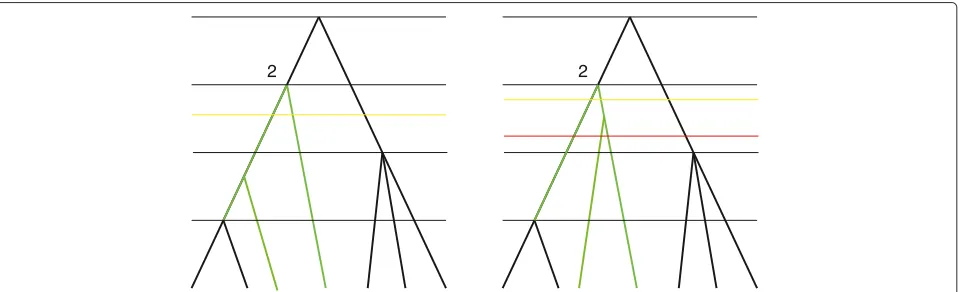
Figure 6Defining matricesmandM.Two trees that resolve a constraint tree from Figure 4 (only resolutions of subtree 2 are shown) and three ways to draw a horizontal line. The yellow lines correspond to the minimal number of intersections and the red line, to maximal. Thus,m2,2=2 and
treei is the subtree which is induced by nodei and its children. Since leaves in subtrees are now ranked, we need more parameters to encode the tree. Letn =[ni,j] be a
matrix of sizek×l, whereni,jis the number of leaves of
rankj in subtreei or the number of children of nodei with rankj. Note that if nodeiis a parent of nodejthen ni,r(j)=1 andni,x=0 forx=r(j)and this means that the
parent function is uniquely defined by the matrixnand functionr and the number of resolutions ofT depends only on(n,r).
If a constraint tree has only 2 leaves then there is only 1 tree resolving it:
Fr((2),r0)=Fr((1, 1),r0)=1
withr0mapping 1 to 1.
For the main recursion we need to determine the loca-tion of the last interior node in a resolving tree. As before, this node can be a parent to leaves in different subtrees. Also, since leaves now may have different ranks, the last interior node in a resolving tree may be ranked in different ways with respect to ranks of the leaves. LetNc,x denote
the number of children of nodecwith ranks at leastx, that
is,Nc,x= l
j=x
nc,j. For eachp∈ {r(k)+1,. . .,l}, we define a
setCpof candidate subtrees in which the last node can be placed at levelp, i.e. between the(p−1)th andpth time points.
Cp= {c | Nc,p≥2 andNc,r(c)+1>2}
See Figure 7 for an example of subtree where the last node can be placed between the(p−1)th andpth time points.
For each p and c such that c ∈ Cp, there is a dis-tinct group of resolving trees. The quantity of trees in this group is equal to the number of resolutions of a constraint tree which is defined by matrixnc,p =[nic,,jp] of sizek×p such that
– nci,,jp=ni,jfor1≤i≤kandj<p;
– ncc,,pp=Nc,p−1;
– nci,,pp=Ni,pfori≤kandi=c.
If nodekhas only 2 children then, as before, there is one more group of resolving trees. This group consists of the resolving trees in which the last interior node coincides with nodek. Letn =[ni,j] be a matrix of size(k−1)×r(k) such that
– ni,j=ni,jfor1≤i≤kandj<r(k),
– ni,r(k)=Ni,r(k)for1≤i≤k−1.
r(c)
r(k)
p-1
p
l
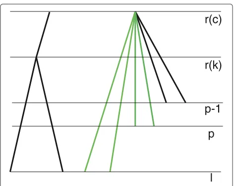
Figure 7Location of a new node between the(p−1)-th andp-th time points.A new node can be placed in subtreecbetween the(p−1)-th andp-th time points if the number of green branches is greater or equal to 2 and the number of all branches in subtreecis greater than 2.
This matrix defines a constraint tree for which the num-ber of resolutions is equal to the numnum-ber of trees in the last group.
Then the main recursion is as follows:
Fr(n,r)=
l
p=r(k)+1
c∈Cp
Nc,p
2
Fr(nc,p,r) (9)
+Fr(n,r|{1,...,k−1}) ifNk,r(k)+1=2;
Fr(n,r)=
l
p=r(k)+1
c∈Cp
Nc,p
2
Fr(nc,p,r) otherwise;
(10)
Using these equations, we can calculate Fr(n,r) for O(m2nk)steps, wheremis the number of sampling points, i.e.,m=l−k. The calculation is described in Appendix 2.
Conclusions
Table 1 The complexity of algorithms
No constraints kconstraints (k=1)
Contemporaneous
sampling O(n) O(nk)
(m=1) Serial sampling
with no sampled O(mn) O(m2nk)
ancestors Serial sampling
with sampled O(mn2)
-ancestors
The table summaries the complexity of the counting algorithms, wherenis the sample size,kis the number of constraints, andmis the number of sampling time-points. We assume thatkis fixed.
These algorithms can be implemented in software for phylogenetic analysis that involves serial sampling scheme or limited prior knowledge about ancestors of particular clades for calculating tree prior distributions.
Appendix 1: Algorithm for counting FRS trees Rewrite equation (2) as follows:
S(n1,. . .,nm)= nm
i=0
A(i,nm−1,nm)S(n1,. . .,nm−1+i)
where A(i,a,b) =
min{a,b−i}
x=0 R(b)
R(i+x) i+x
x
a
x
. Then we can
calculateS(n1,. . .,nm)recursively using Algorithm 3. We
use the notationNj= m
i=j
ni.
Algorithm 3Calculating the number of FRS trees fori=1→N1do
calculateR(i)usingR(i)=R(i−1)i(i−12 )
end for
forj=2→mdo
calculateA(0,nj−1,nj),. . .,A(nj,nj−1,nj)
calculateS(n1,. . .,nj) forα=1→Nj+1do
calculate A(0,nj−1,nj + α),. . .,A(nj + α,nj−1,
nj+α)
calculateS(n1,. . .,nj+α) end for
end for
At each step j > 1 of the algorithm, we calculate S(n1,. . .,nj+α)for 0 ≤ α ≤ Nj+1. We skip stepj = 1 and do not calculateS(n1+α)for 0 ≤ α ≤ N2because S(x) =R(x)and we have already calculated all the neces-saryR(x). Further, for calculating eachS(n1,. . .,nj+α),
we need to calculate the coefficientsAand this is the most expensive part of the algorithm. So, at each stepj>1, we need to calculateA(i,nj−1,nj+α)for 0≤i≤nj+αand
0≤α≤Nj+1.
First, we calculate these values forα=0. Denote
B(i,a,b,x)= R(b) R(i+x)
i+x
x
a x
, forx≤aandi+x≤b
then
A(i,a,b)=
min{a,b−i}
x=0
B(i,a,b,x)
where 0 ≤ i ≤ b, a = nj−1, and b = nj. When
i is fixed, calculation of A(i,nj−1,nj) requires values of
B(i,nj−1,nj,x) for 0 ≤ x ≤ min{nj−1,nj −i}. Rewrite
this as B(nj −β,nj−1,nj,x) for 0 ≤ x ≤ min{nj−1,β} with β = nj −i. Now we can calculate these values for
0 ≤ β ≤ nj and, hence, for 0 ≤ i ≤ nj using recursive
equations:
B(nj,nj−1,nj, 0)=1
B(nj−(β+1),nj−1,nj,x)
= (nj−(β+1)+x)(nj−β)B(nj−β,nj−1,nj,x) 2
(11)
B(nj−(β+1),nj−1,nj,(β+1))
= (nj−β)(nj−1−β)B(nj−β,nj−1,nj,β)
(β+1)2 (12)
We use equation (11) for 0 ≤ x ≤ min{nj−1,β}. If min{nj−1,β + 1} = min{nj−1,β} and therefore
min{nj−1,β +1} = min{nj−1,β} +1 = β +1 then we
also use equation (12). The cost of this calculation is domi-nated by the number of the summandsB(nj−β,nj−1,nj,x)
for 0≤x≤min{nj−1,β}and 0≤β ≤nj. This number is
O(n2j).
Now we need to calculateA(0,nj−1,nj+α),. . .,A(nj+α,
nj−1,nj+α)for 1≤α ≤Nj+1. HavingA(0,nj−1,nj+α),
. . .,A(nj+α,nj−1,nj+α)calculated (note that we have
already calculated these values forα=0), we can calculate A(0,nj−1,nj+(α+1)),. . .,A(nj+(α+1),nj−1,nj+(α+1))
A(i,a,b+1)= ⎧ ⎪ ⎪ ⎨ ⎪ ⎪ ⎩
(b+1)b
2 A(i,a,b)+
b+1
i
a b+1−i
ifb−i<a,
(b+1)b
2 A(i,a,b) ifa≤b−i and
(13)
A(b+1,a,b+1)=1
where 0≤i≤b,a=nj−1, andb=nj+α.
Moreover, for eachα, we can optimize calculation of the second summands in the first case of equation (13) using recursion
nj+α
i+1
nj−1
nj+α−(i+1)
= (nj+α−i)2 (i+1)(nj−1−nj−α+i+1)
nj+α
i
nj−1
nj+α−i
(14)
To apply this recursion we need an initial value. This value depends onnj−1,nj, andα and, since only the first
case of equation (13) contains the second summand, it is not necessary the value of this summand fori=0. There are 3 cases for calculation of all the initial values that are necessary at stepj.
Case 1: Nj<nj−1. That means that we use the first case of equation (13) for allα. In this case, for allα, the initial value for recursion (14) is the value of the second summand in (13) wheni=0. So we need to calculatenj+0α nj−1
nj+α+0
for
1≤α≤Nj+1and those are nj−1
nj+1
,. . ., nj−1 nj+Nj+1
. This takesO(Nj)steps.
Case 2: nj+α0=nj−1for someα0∈ {0,. . .,Nj+1}. If
α0>0then, for allα≤α0, we use the first case of (13) and therefore we need to calculate nj−1
nj+1
,. . .,nj−1 nj+α0
, this takesO(α0)steps. For allα > α0, we use the second case first and, starting fromi=α−α0, we use only the first case. So we need to calculate
nj+α α−α0
nj−1
nj+α−(α−α0)
forα∈ {α0+1,. . .,Nj+1},
which arenj−1+1 1
,. . .,nj−1+(Nj+1−α0)
(Nj+1−α0)
. This takesO(Nj+1−α0)steps. In total, we have O(Nj+1)steps.
Case 3: nj−1<nj. That means that, for allα, we use the
second case first and, starting from
i=nj+α−nj−1, we use only the first case.
Calculatenjnj+1−
1
,. . .,nj+Nj+1 nj−1
for O(nj−1+Nj+1)steps.
Each case costs at most O(Nj). Provided that the
ini-tial values are calculated, the cost of the rest calculation at stepjis dominated by the number of the coefficients
A(i,nj−1,nj+α)for 0≤i≤nj+αand 1≤α≤Nj+1and it isO(Nj2). Summing upO(n2j),O(Nj−1), andO(Nj2)gives
us the cost of each stepj, which isO(Nj2). Since 1<j≤m and calculation ofR(i)for 0≤i≤N1=ntakesO(n), the algorithm doesO(mn2)steps in total.
Appendix 2: Algorithm for counting fully ranked resolutions of a fully ranked constraint tree
The algorithm for counting resolutions of a constraint tree requires a few changes to count resolutions of a fully ranked constraint tree. Recall that, at each step s, we calculated the setSswhich consists of the numbers of
res-olutions of intermediate trees withsleaves. To construct Ss, for each element ofSs−1, we proposed a collection of
tuples that may define intermediate trees with s leaves. To accept eligible tuples we defined two matricesmand M. The general scheme for counting resolutions of a fully ranked constraint tree is the same. However, we need to define matricesmandMfor a fully ranked constraint tree and describe the procedure of proposing new tuples. The procedure becomes more technical because of additional ranking.
We will calculate Sr(n,r) for the corresponding fully
ranked constraint treeT. Let
ai,j= |{x | nodeiis a parent of node xandr(x)≤j}|
for 1≤i ≤kandr(i)≤j≤ l−1, i.e.,ai,jis the number
of interior nodes that are children of nodeiand have rank at mostj. Define two matricesmandMof sizek×(l−1) such that
Mi,j=Ni,j+1 and mi,j=
⎧ ⎪ ⎨ ⎪ ⎩
2 ifai,j=0;
1 ifai,j>0 andMi,j>0;
0 otherwise.
As before, if we consider a horizontal line that is strictly between the horizontal line that passes through the nodes of rankjand the horizontal line that passes through the nodes of rank(j+1)then these matrices determine the minimal and maximal possible numbers of intersections of this line with branches of subtreei.
Letx=[xi,j] be a matrix of sizet×q, wheret≤ kand
q≤l, andt= {1,. . .,t}. A tuple(x,r|t)is eligible if
– xi,j=ni,jfor1≤i≤tand1≤j<q, and
Having an intermediate tree withs−1 leaves, we need to consider all the possible ways to transform this tree to a tree withsleaves. First we need to add a new leaf to some subtree. We give the highest rank to this leaf. After that we may add new time points below the last time point. If we add new time points, we should rerank the leaves with the highest rank such that the new tree has enough leaves at each time point. Let x =[xi,j] be a matrix of
sizet× qfort ≤ kandq ≤ l. This matrix represents an intermediate tree withs−1 leaves. Suppose we add a new leaf to subtree i0, where 1 ≤ i0 ≤ t. Let q0 be the number of time points in a new tree and, therefore, q≤q0≤r(t+1)(orq≤q0≤lift=k). Define a func-tionaddone((x,r|t),i0,q0) which returns a tuple(x,r|t), wherex =[xi,j] is a matrix of sizet×q0such that
– xi0,q0 =xi0,q−
q0−1
j=q ni0,j+1,
– xi,q0 =xi,q−jq=0−1q ni,jfori=i0, – xi,j=xi,jfor1≤i≤tandj<q, and
– xi,j=ni,jfor1≤i≤tandq≤j<q0.
If this tuple is eligible then it represents a new interme-diate tree withsleaves.
At each step sof the algorithm, for each tuple (x,r|t) such that Fr(x,r|
t) ∈ Ss−1, we need to propose a
col-lection of new tuples. The first part of this procedure is Algorithm 4. To stop the procedure, when we recognise that a new tree can not havextime points, we use a pred-icateext(x)which is true if we can extend the number of time points in a new tree tox. The number of time points in a new tree can not always be extended to any arbitrary number because there may not be enough leaves of the highest rank to rerank them in such a way that there will beni,jleaves of each new rankj. Soext(q)is always true
because the tree to which we add a new leaf already hasq time points.
Algorithm 4 Working with a tuple (x,r|t) such that Fr(x,r|t)∈Ss−1(part 1)
q0=q
whileq0≤r(t+1)(orq0≤lift=k) andext(q0)do
fori=1→tdo
(x,r|t)=addone((x,r|t),i,q0)
ifeligible((x,r|t))then
calculateFr(x,r|t)and add it toSs end if
ifall the proposed tuples were not eligiblethen
ext(q0+1)=false
end if
q0=q0+1
end for end while
Ift<kthen the proposing procedure contains the sec-ond part. In this case, we also can increase the number of leaves in an intermediate tree by adding a new subtree. That means that one of the leaves of the tree becomes a parent to two new leaves. Again we may add new time points. Letq0be the number of time points in a new tree and, therefore,r(t+1) < q0 ≤ r(t+2)(orr(t+1) < q0 ≤ l when t +1 = k). We define another function addconstraint((x,r|t),q0)which returns a tuple(x,r|t+1), wherex =[xi,j] is a matrix of size(t+1)×q0such that
– xt+1,q0 =2−q0−1
j=r(t+1)+1nt+1,j,
– xt+1,j=nt+1,jfor1≤j<q0,
– xi,q0 =xi,q−qj=0−1q ni,jfor1≤i≤t,
– xi,j=xi,jfor1≤i≤tandj<q, and – xi,j=ni,jfor1≤i≤tandq≤j<q0.
This tuple defines a new tree if it is eligible. The second part of the procedure is Algorithm 5. The values ofq0and ext(q0)are as after running Algorithm 4.
Algorithm 5 Working with a tuple (x,r|t) such that Fr(x,r|t)∈Ss−1(part 2)
whileq0 ≤ r(t+2)(orq0 ≤ lwhent+1 = k) and ext(q0)do
(x,r|t+1)=addconstraint((x,r|t),q0)
ifeligible(x,r|t+1)then
calculateFr(x,r|t+1)and add it toSs else
ext(q0+1)=false
end if
q0=q0+1
end while
Finally, as before, the main algorithm calculates setsSs
recursively for 0 ≤ s ≤ n, where n is the number of leaves in a constraint treeT, and a unique element ofSnis
Sr(n,r).
Letmbe a number of sampling points, i.e.,m=l−k.
Proposition 2.If k is fixed then the algorithm does at most O(m)steps for each eligible tuple.
Proof. Let(x,r|t)be an eligible tuple. First, having all the necessary summands for equations (9) and (10), we need to calculateFr(x,r|
t). This takes at mostO(t×[r(t+1)− r(t)]) steps. Since we assume k is a constant and since t≤kandr(t+1)−r(t)≤m, it isO(m). Second, we need to perform the procedure of proposing new tuples for this tuple. The most expensive part here is calculation of the last columns of matricesx because it involves calculation of the sums q0−1
xi,q−
q0−1
j=q ni,jfor 1≤i≤tat each stepq0, we can opti-mise these calculations. Then it takesO(t×(q−r(t+2)) steps and it isO(m)again.
Proposition 3.If k is fixed then the algorithm has O(m2nk)time complexity.
Proof.Letixbe such a number thatr(ix)≤x<r(ix+1).
Then the number of eligible tuples is
l−1
j=1
ij
i=1
(Mi,j−mi,j+1)
Note that
Mi,j−mi,j+1≤Ni,j+1≤Ni,r(i)+1+1=bi+1
whereb1+. . .+bk=n+k−1. Then
l−1
j=1
ij
i=1
(Mi,j−mi,j+1) < (l−1)(b1+1) . . . (bk+1)
< (l−1)(n k)
k =O(mnk)
From this and Proposition 2, it follows that the algo-rithm does at mostO(m2nk)steps.
Competing interests
The authors declare that they have no competing interests.
Authors’ contributions
The authors equally contributed to conceive the work. AG drafted the manuscript and DW and AJD revise it. All authors read and approved the final manuscript.
Acknowledgements
AJD was partially funded by a Rutherford Discovery Fellowship from the Royal Society of New Zealand.
Author details
1Department of Computer Science, The University of Auckland, Auckland, New Zealand.2Allan Wilson Centre for Molecular Ecology and Evolution, University of Auckland, Auckland, New Zealand.
Received: 15 February 2013 Accepted: 8 October 2013 Published: 28 October 2013
References
1. Yang Z, Rannala B:Bayesian phylogenetic inference using DNA sequences: a Markov chain Monte Carlo method.Mol Biol Evol1997, 14(7):717–724.
2. Yang Z, Rannala B:Bayesian estimation of species divergence times under a molecular clock using multiple fossil calibrations with soft bounds.Mol Biol Evol2005,23:212–226.
3. Heled J, Drummond A:Tree priors for relaxed phylogenetics and divergence time estimation.Syst Biol2012,61:138–149.
4. Rodrigo AG, Felsenstein J:The Evolution of HIV. Baltimore: Johns Hopkins Univ Press; 1999.
5. Drummond A, Pybus O, Rambaut A, Forsberg R, Rodrigo A:Measurably evolving populations.Trends Ecol Evol2003,18:481–488.
6. Felsenstein J:Inferring Phylogenies. Sunderland: Sinauer Associates; 2004.
7. Murtagh F:Counting dendograms: a survey.Discrete Appl Math1984, 7:191–199.
8. Gordon AD:A review of hierarchical classification.J R Stat Soc A1987, 150(2):119–137.
9. Semple C, Steel M:Phylogenetics. New York: Oxford University Press; 2003. 10. Griffiths RC:Counting genealogical trees.J Math Biol1987,25:423–431. 11. Felsenstein J:The number of evolutionary trees.Syst Zool1978,
23:27–33.
12. Stadler T:Sampling-through-time in birth-death trees.J Theor Biol 2010,267(3):396–404.
13. Stadler T, Kouyos RD, von Wyl, V, Yerly S, Böni J, Bürgisser P, Klimkait T, Joos B, Rieder P, Xie D, Günthard HF, Drummond A, Bonhoeffer S, the Swiss HIV Cohort Study:Estimating the basic reproductive number from viral sequence data.Mol Biol Evol2012,29:347–357.
doi:10.1186/1748-7188-8-26
Cite this article as: Gavryushkina et al.: Recursive algorithms for phylogenetic tree counting.Algorithms for Molecular Biology20138:26.
Submit your next manuscript to BioMed Central and take full advantage of:
• Convenient online submission
• Thorough peer review
• No space constraints or color figure charges
• Immediate publication on acceptance
• Inclusion in PubMed, CAS, Scopus and Google Scholar
• Research which is freely available for redistribution