Online Stator and Rotor Resistance Estimation Scheme Using Sliding Mode Observer for Indirect Vector Controlled Speed Sensorless Induction Motor

(1)

http://www.sciencepublishinggroup.com/j/ajcst doi: 10.11648/j.ajcst.20190201.11

ISSN: 2640-0111 (Print); ISSN: 2640-012X (Online)

Online Stator and Rotor Resistance Estimation Scheme

Using Sliding Mode Observer for Indirect Vector Controlled

Speed Sensorless Induction Motor

Djamila Cherifi

*

, Yahia Miloud

Electrical Engineering Department, Dr Moulay Tahar University, Saida, Algeria

Email address:

*_{Corresponding author}

To cite this article:

Djamila Cherifi, Yahia Miloud. Online Stator and Rotor Resistance Estimation Scheme Using Sliding Mode Observer for Indirect Vector Controlled Speed Sensorless Induction Motor. American Journal of Computer Science and Technology. Vol. 2, No. 1, 2019, pp. 1-8. doi: 10.11648/j.ajcst.20190201.11

Received: November 17, 2018; Accepted: December 20, 2018; Published: January 29, 2019

Abstract:

Recently, many works have been made to improve the performance of sensorless induction motor drives. However, parameter variations and low-speed operations are the most critical aspects affecting the accuracy and stability of sensorless drives. This work presents a sensorless vector control scheme consisting of the first hand of a velocity estimation algorithm that overcomes the need for sensor velocity and secondly a robust variable structure control law that compensates for the uncertainties present in the system. Simulation results confirm the efficacy of the proposed approach.

Keywords:

Induction Motor Drive, Indirect Field Oriented Control, Sensorless, Sliding Mode Observer, Simultaneous Parameter Estimation

1. Introduction

The induction motor (IM) is widely used in industry because of its advantages such as reliability, efficiency, and low cost in comparison to other motors used in similar application [1]. The dynamic model of induction motor is precisely nonlinear, so having control over induction motor is a challenging problem which attracted much attention. The vector controlled method is generally used due to its simplicity and fast response. The use of vector controlled induction motor drives allows obtaining several advantages compared to the DC motor in terms of robustness, size, lack of brushes, and reducing cost and maintenance. It achieves effective decoupling between torque and flux, [2-4].

The speed of an induction motor is usually measured by using a speed sensor. But the speed sensors are not suitable under varying environmental conditions, as the measurement suffers due to large mechanical shocks. It also reduces the reliability and increases the cost of the drive. In recent years sensorless induction motor drives have been widely used. But sensorless speed FOC induction motor drive are sensitive to the motor parameter variations, especially to the stator and

rotor resistances that change with temperature and skin effects, [5, 6]. It is clear that when this parameters varies, decoupling between the flux and torque components of stator currents is lost and hence the operational performance of the machine deteriorates. However, when a very high accuracy is desired, the performance of speed estimation is not good particularly at low speeds, [7, 8, 9]. To solve this problem, this paper proposes a method for both rotor speed identification with stator and rotor resistance estimation in sensorless induction motor drives based on sliding mode observer.

This paper is organized as follows. Section 2 shows the dynamic model of induction motor. Sliding mode observer will be described in Section 3. The proposed solution will be presented in Section 4. In Section 5, results of simulation tests are reported. Finally, Section 6 draws conclusions.

2. Dynamic Model of Induction Motor

(2)













− − = − − − = − + − = + + − − − = + + + + − = r J f l T em T J p dt r d rq r T rd r s sq i r T m L qr dt d rq r s rd r T sd i r T m L dr dt d sq V A rq r T s L r L m L rd r A sq i A sd i s qs i dt d sd V A rq r A rd r T r L s L m L sq i s sd i A ds i dt d ω ω φ φ ω ω φ φ ω ω φ φ φ σ φ ω ω φ ω φ σ ω ) ( 1 ). ( . ). ( 1 . 3 . . . . 2 . 1 . 3 2 . . . . . 1 (1) Where       ₋ + = r s s T L R A . 1 . 1

σ

; s r

m L L L A . .

2 =_σ

s L A

. 1

3=_σ ;

r s m L L L2 1 − = σ

;ωg =ωs−ωr

) .i -.i ( 2 3 sd rq sq rd φ φ r m em L L P T =

ωs and ωr are the electrical synchronous stator and rotor speed; σ is the linkage coefficient, and Tris the rotor time constants.

3. Sliding Mode Observer

A sliding-mode observer is an observer whose gain-corrector term contains the discontinuous function: sign. Sliding modes are control techniques based on the theory of systems with variable structure, [10].

A sliding-mode observer is written in the form, [11]:

) ˆ ( ˆ ) ˆ ( ) , ˆ ( ˆ

ξ

h y y y sign u f = − Λ + = ɺ (2) With

ξ

ˆ

_{: Estimated state}

Λ

: Matrix Gain of the observer

(.)

f

: Nonlinear function of state evolution

(.)

h

: Nonlinear output function

y

and

y

ˆ

: Outputs measured and estimated.

The sliding mode observer consists of stabilizing the error dynamics of the states to be estimated, which amounts to, [11]:

- Determine a slip surface on which the error of the

estimate of the output is zero.

- Establish the slip conditions (calculation of the observer's gains for which all the trajectories of the system move towards the sliding surface (attractiveness) and remain there (invariance).

The observer is only a copy of the original system to which one adds the control gains with the terms of commutation; thus, ) ˆ ( ˆ ˆ ˆ s s i i sign K Bu x A dt x d − + +

= (3)

The sliding surfaces are defined by:

        − − =       = β β α α s s s s i i i i S S S ˆ ˆ 2 1 (4)

The difference between the models (system and observer) generates a state model of the error is given as follows:

) ˆ ( ˆ Ksign i_s i_s x A Ae dt de − + ∆ +

= (5)

The conditions of the sliding mode, in terms of convergence towards the surface and invariance on the same surface, make it possible to write:

0 , 0 = = dt de

e_i i (6)

And so the equation of state (5) becomes:

LH A i A e A e dt d H A i A e A r s r s + ∆ + ∆ + = − ∆ + ∆ + =

φ

φ φ φ ˆ ˆ ˆ ˆ 0 22 21 22 12 11 12 (7)

(3)

The modeling error, or variation of A, is considered to be due to the only variation of the parameter

ω

, hence the formulations:         ∆ ∆ − = ∆ J J A ω ε ω 0

0 _;

∆

ω

=

ω

ˆ

−

ω

_;

      − = 0 1 1 0 J

The substitution in equations (7) gives:

H J e

A −∆ _r−

= φ

εω

φ ˆ

0 ₁₂ (8)

LH J e A e dt d r r + ∆ + = _φ

ω

φ

φ 22 ˆ (9)

From equation (8), he comes:

H A J A

e =∆ r ₁₂−1

φ

ˆ_r+ ₁₂−1

ε

ω

φ (10)

φ

e

, of the expression (10) introduced in equation (9) gives:

LH J H A A J A e dt d r r r

r ₊ ₊_∆ ₊

∆

=

φ

− −

ω

φ

ε

ω

φ ( ˆ 121 ) ˆ

1 12

22 (11)

Knowing that,

A

₂₂

=

−

ε

A

₁₂ Equation (11) becomes simpler and becomes:

) ( 1sign ei

K H e dt d Λ − = Λ =

φ (12)

With

Λ

=

(

L

−

ε

I

)

and

m r s L L L σ ε =

With regard to the determination of k1 and k2 one must

check the condition of Popov

S

.

S

ɺ

<

0

, to ensure the stability of the flow observer. As a result, the equation of the current error in the following form must first be explained:

      − − +             − +             − − =       ) .( ) .( . . 0 0 2 2 1 1 4 3 2 3 3 2 2 1 1 1 2 1 e sign k e sign k e e e e e e dt d γ γ γ γ γ γ (13) With r r s m s s L L L L R η σ σ γ . . . 2

1= +

; r r s m L L L η σ γ . . 2 = ; r r s m L L L ω σ γ . . 3=

And since the state variables

φ

_r_α(t),

φ

_r_β(t) are naturally bounded, we consider two positive parameters such as

1

η

φrα < and

φ

rβ <

η

2

Assuming moreover that both parameters

η

₁ and

η

₂satisfy the following two equations:

(

η φα

)

_σ ω

(

η φβ

)

η σ η σ σ

ρ r r

r s m r r r s m r r s m s s L L L L L L e L L L L R ˆ . . . ˆ . . . . . . 2 1 1 2

1  + + + +

       + >

(

η φβ

)

_σ ω

(

η φα

)

η σ η σ σ

ρ r r

r s m r r r s m r r s m s s L L L L L L e L L L L R _ˆ . . . ˆ . . . . .

. 2 2 1

2

2  + + + +

     + >

So if we take,

k

₁

=

ρ

₁

+

c

₁ and

k

₂

=

ρ

₂

+

c

₂

With c1 and c2 are two positive constants.

4. Simultaneous Estimation of Rotor

Speed and Stator Resistance by Sliding

Mode Observer

The estimation method hereafter estimates the rotor speed of the induction motor and the stator resistance of the motor at the same time. Thus, this method improves the estimation accuracy, reliability and robustness of the induction motor speed identification system.

The state model of the error is given as follows, [12-14].

) ˆ ( ˆ Ksign i_s i_s x A Ae dt de − + ∆ +

= (14)

The state model of the error is given as follows With: T i

e

x

e

=

ˆ

−

=

[

_φ

]

State error, state estimation error

A

=

−

∆

ˆ

_{Modeling error}

s s

i

e

=

ˆ

−

Current error, stator current estimation error

r r

e

_φ

=

φ

ˆ

−

φ

Flow error, rotor flow estimation error













∆

=

∆

22 21 12 11

A

(4)

        ∆ ∆ − ∆ − = ∆ J J I L R A _s s ω ε ω σ 0 (16) With

ω

=

−

∆

ˆ

; ∆Rs=Rˆs−Rs;

m r s L L L σ ε= ;       − = 0 1 1 0

J ; 

     = 1 0 0 1 J

4.1. Stability of Identification System

Popov's theory of hyper-stability is applied here to examine the stability of the proposed identification system. This requires that the error system and the feedback system be derived so that the theory could be applied.

The authors in [8, 15-17] proposed that the actual and estimated rotor fluxs are the same, hence the error equation (14) is as follows:

r

s A

i A

z=∆ ₁₁ˆ +∆ ₁₂

φ

ˆ (17)

Or

)

ˆ

(

1

sign

i

s

i

s

K

z

=

−

Substitute

∆

A

11_and

∆

A

12_{in (16) becomes:}

r s

s

s _I_i _J

L R z φ ε ω σ ˆ ˆ ∆ − ∆ −

= (18)

We pose

s s

i L L₁ 1 _ˆ

      =

σ

, r

J L

φ

ε

ˆ 2       = r s

L

R

L

z

=

−

₁

∆

−

₂

∆

ω

(19)

Popov's criterion of equation (18) writes as follows:

2 0

.

1

y

dt

W

z

S

t T

−

≥

=

∫

(20)

with is y= const

r

s

L

R

L

W

=

−

₁

∆

−

₂

∆

ω

, which represents the non-linear block

dt

L

R

L

z

W

z

S

r s t T t T

)

(

.

2 1 0 0 1 1

ω

∆

−

∆

−

=

∫

(21)

Substitute the equations (IV.39), it comes:

dt

J

z

i

L

R

z

W

z

S

t r r T s s s T t T

∫

=

−

∆

−

∆

=

1 1 0 0

ˆ

.

φ

ε

ω

σ

(22)

dt

J

z

dt

i

L

R

z

S

t r r T t s s s T

∫













∆

−

+













∆

−

=

1 1 0 0

ˆ

φ

ε

ω

σ

(23)

2 2 1

y

S

=

+

≥

−

(24)

2 0 1 1

ˆ

y

dt

i

L

R

z

S

t s s s T

−

≥













∆

−

=

∫

σ

(25)

2 0

2

1

ˆ _dt _y

J z S t r r T − ≥         _∆ − =

∫

φ ε ω (26)

The condition (24) is verified by equalization of (25) and (26) with the adaptation mechanism is given by (27), (28) for speed estimation and online identification of the stator resistance respectively:

∫

− − −

=K k sign i_s i_s _r k signi_s i_s _r dt

r [ (ˆ )ˆ (ˆ )ˆ ]

ˆ _ω ₁ _α _α φ_β ₂ _β _β φ_α

ω (27)

∫

− − −

=K k sign i i i k signi i i dt

R_s _R _s _s _s _s _s _s

s ] ˆ ) ˆ ( ˆ ) ˆ ( [ ˆ 2

1 α α α β β β (28)

Where

s R

K

(5)

4.2. Estimation of Rotor Resistance

To improve the performance and simplify the vector control and reduce its cost, we will base this part on a hypothesis to deduce the value of the rotor resistance estimate from the estimation of the stator resistance. Still, it is assumed that the motor windings are almost at the same temperature, and neglecting the skin effect, the resistances will vary proportionally.

The rotor resistance estimate can be determined by the following relation, [18]:

n s

n r s r

R R R R

. .

. ˆ

ˆ ₌ ₍₂₉₎

5. Simulation Results and Discussion

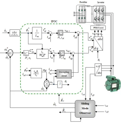
To demonstrate the faisability of the proposed estimation algorithm, and incorporated into a speed control system of a IM with indirect oriented rotor flux, the simulation of the complete system, figure 1 was carried out using different of cases that will be presented and discussed next.

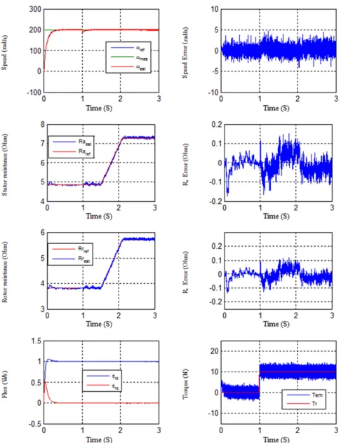
The simulation results (Figure 2), show the simultaneous

estimation of the speed and two resistors (stator and rotor) It is clear that:

The estimated resistances converge to the nominal resistances quickly and with great accuracy, or the estimation error is acceptable after a very short transient regime.

The injection of these values into the flux observer keeps the performances of the flux observer and the vector control, in fact all the basic magnitudes of the machine (speed, rotor flux, stator currents, and the torque ) converge to their nominal values.

So we can say that all the parameters are identical (resistances of the motor and the observer).

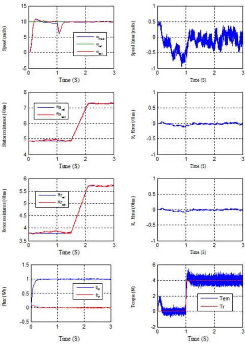
- Low speed operation

Figure 3 illustrates the simulation results of the Speed Sensorless Vector Control based on estimation of the speed of rotation, Rr and Rs simultaneously, for a low speed reference (10 rad / sec) and application of a resistant torque at t=1s.

Note that the convergence of the resistive parameters is always ensured. So we can conclude that this observer can work satisfactorily in the various conditions, either that it is the heating of the resistances or the low speed drive.

(6)

(7)

(8)

6. Conclusions

This paper proposes the simultaneous estimation of rotor speed with rotor and stator resistance for speed sensorless control of induction motor. This estimation technique mainly responds to the most critical needs of the induction machine control laws in terms of parametric robustness and ensures smooth operation over the entire speed range. It is used to process the estimation of the following quantities: the rotor flux, the rotor resistance, the stator resistance and the speed of rotation. Several ideas have been exploited to meet these needs.

The analysis of the results obtained shows that this estimation technique makes it possible to obtain a flow and torque decoupling comparable to that of a separate excitation DC machine. During the tests carried out, we notice the superiority of the sliding mode observer in terms of robustness even with respect to strong disturbances (load and resistances) with a fairly fast tracking dynamics.

Appendix

Induction Motor Parameters

1.5 Kw, 1420 rpm, 380 V, 3.7A, 50 Hz,

Rr =3.805Ω, Rs =4.85Ω, Ls =274 mH, Lr =274 mH J =

0.031 kg.m2, F=0.00114kg.m2/s.

References

[1] Zicheng Li, Zhouping Yin, Youlun Xiong and Xinzhi Liumm " Rotor Speed and Stator Resistance Identification Scheme for Sensorless Induction Motor Drives"m TELKOMNIKA, Vol.11, No.1, January 2013, pp. 503~512.

[2] E¸ s. Ozsoy, M. G. Okasan, S. Bogosyan, "Simultaneous rotor and stator resistance estimation of squirrel cage induction machine with a single extended kalman filter", Turk J Elec Eng & Comp Sci, Vol.18, No.5, 2010

[3] DJ. Cherifi, Y. Miloud, A. Tahri, " New Fuzzy Luenberger Observer for Performance Evaluation of a Sensorless Induction Motor Drive", International Review of Automatic Control (I. RE. A. CO.), Vol. 6, n. 4 July 2013.

[4] T. ORLOWSKA-KOWALSKA and G. TARCHALA, "Unified approach to the sliding-mode control and state estimation– application to the induction motor drive", BULLETIN OF THE POLISH ACADEMY OF SCIENCES TECHNICAL SCIENCES, Vol. 61, No. 4, 2013.

[5] A. M. El-Sawy, Yehia S. Mohamed and A. A. Zaki, "Stator Resistance and Speed Estimation for Induction Motor Drives As Influenced by Saturation", The Online Journal on Electronics and Electrical Engineering (OJEEE).

[6] R. Tak, S. Y Kumar and B. S. Rajpurohit, "Estimation of

Rotor and Stator Resistance for Induction Motor Drives using Second order of Sliding Mode Controller", Journal of Engineering Science and Technology Review 10 (6) (2017) 9 - 15.

[7] Y. Agrebi Zorgani, Y. Koubaa, M. Boussak, "Simultaneous Estimation of Speed and Rotor Resistance in Sensorless ISFOC Induction Motor Drive Based on MRAS Scheme", XIX International Conference on Electrical Machines - ICEM 2010, Rome.

[8] M. S. Zaky, M. M. Khater, H. Yasin, and S. S. Shokralla, “Speed and Stator Resistance Identification Schemes for a Low Speed Sensorless Induction Motor Drive”, 2008 IEEE. [9] M. AKTAS, H. I. OKUMUS, "Stator resistance estimation

using ANN in DTC IM drives", Turk J Elec Eng & Comp Sci, Vol.18, No.2, 2010.

[10] G. Tarchala, T. O-Kowalska, “Sliding Mode Speed Observer for the Induction Motor Drive with Different Sign Function Approximation Forms and Gain Adaptation », PRZEGLĄD ELEKTROTECHNICZNY, ISSN 0033-2097, R. 89 NR 1a/2013.

[11] K Kouzi, M-S. Nait –Said, M. Hilairet, E. Berthlol, “A robust fuzzy speed estimation for vector control of an induction motor”, 2009 IEEE

[12] F. Mellah, M. Chenafa, A. Bouhenna, A. Mansouri, “Passivity Control with sliding mode observer of induction motor”, Przegląd Elektrotechniczny (Electrical Review), ISSN 0033-2097, R. 87 NR 7/2011.

[13] A. Farrokh Payam, M. Jalalifar, “Robust Speed Sensorless Control of Doubly- Fed Induction Machine Based on Input-Output Feedback Linearization Control Using a Sliding-Mode Observer”, 0-7803-9772-X/06/$20.00 ©2006 IEEE.

[14] Hongryel Kim, Jubum Son, and Jangmyung Lee, “A High-Speed Sliding-Mode Observer for the Sensorless High-Speed Control of a PMSM”, IEEE Transactions on Industrial Electronics, VOL. 58, NO. 9, September 2011.

[15] M. S. Zaky, "A stable adaptive flux observer for a very low speed-sensorless induction motor drives insensitive to stator resistance variations", Ain Shams Engineering Journal (2011). [16] G. Venkatesh, S. VijayaBhaskar, B. Mohan Reddy, “Efficient

Speed Estimation of an Induction Motor Drive Using Sliding Mode Observer Algorithm”, International Journal of Engineering Research & Technology October - 2013.

[17] P. Dharani, D. Nagaraju, R. Nagesh,”Wide-Speed-Range Estimation with Online Parameter Identification Schemes of Sensorless Induction Motor Drives”, International Journal of Emerging Research in Management &Technology October 2013.