On Efficient Iterative Numerical Methods for Simultaneous Determination of all Roots of Non-Linear Function

(1)

On Efficient Iterative Numerical Methods for

Simultaneous Determination of all Roots of

Non-Linear Function

1_{Mudassir Shams,}1_{Nazir Ahmad Mir,}2_{Naila Rafiq}

1_{Department of Mathematics and Statistics, Riphah International University I-14, Islamabad 44000, Pakistan} 2_{Department of Mathematics, NUML, Islamabad, Pakistan}

[email protected], [email protected], [email protected]

Abstract: We construct a family of two-step optimal fourth order iterative methods for finding single root of non-linear equations. We generalize these methods to simultaneous iterative methods for determining all the distinct as well as multiple roots of single variable non-linear equations. Convergence analysis is present for both cases to show that the order of convergence is four in case of single root finding method and is twelve for simultaneous determination of all roots of non-linear equation. The computational cost, Basin of attraction, efficiency, log of residual and numerical test examples shows, the newly constructed methods are more efficient as compared to the existing methods in literature.

Keywords: Single roots; Distinct roots; Multiple roots; Optimal order; Non-Linear equation; Iterative methods; Simultaneous Methods; Basin of attraction; Computational Efficiency

Introduction

To solve non-linear equation

f x( )=0 (1) is the oldest problem of science in general and in mathematics in particular. These non-linear equations have a diverse application in many areas of science and engineering. Several iterative methods have been used to find the roots of non-linear equation (1), using different techniques such as Decomposition methods, Homotopy analysis method, Variation iteration methods and modification in Newton Raphson method etc. All these methods are used to approximate one root at a time. But mathematician are also interested in simultaneous finding of all roots of non-linear equation because simultaneous iterative methods are very popular due to their wider region of convergence, are more stable as compared to single root finding methods and implemented for parallel computing as well. More detailed on single as well as simultaneous determination of all roots can be found in [1-1011-13, 15, 22, 24-30] and reference cited there in. The most famous of single root finding method is the classical Newton -Raphson method:

( ) , ( 1, 2,...) ( )

i

i i

i

f x

y x i

f x

= − = (2)

Methods (2) is optimal having efficiency1.43 . Using Weierstrass’ Correction [11]

1 ( ) ( )

( ) ,

( ) ₍ ₎

i

i n

i j

j i j

f x f x

w x

f x _x _x

 =

= =

 − (3)

in (2) then, we get classical Weierstrass - Dochive methods to approximate all roots of (1) is:

(2)

1 ( ) , ( ) i

i i n

i j j i j f x y x x x  = = −  − (4)

The main aim of this paper is to construct family of optimal fourth order method and then generalize it into simultaneous iterative methods for finding all roots of non-linear equation (1).

Constructions of Method and Convergence

Analysis

Here, we present some optimal fourth iterative methods for finding roots of non-linear equation (1) are:

Jarrat et al. [16] suggest the following optimal fourth order methods (abbreviated as JM):

(

)

( ) 2 3 ( ) ( ) ₂ ( ) ( )

3 3 ( ) ( ) ( )

,

1 .

i i

i i i

i i

i

f x

i i

f x

f x f y f x

i i f y f x

f x y x z x    −   −   = −   = − −   (5)

Siyyam et al. [17] present the folloeing optimal fourth order iterative method (abbreviated as SM):

( ) ( )

2 ( ) ( ) ( )(1 ( )) ( ) 2 ( )

,

.

i i

i i i i

i

f x

i i

f x

f x G u y x G u f x

i i f x y x z y    + − +  = −   = −   (6)

where (₍ i)₎ i

f y f x

u= and 2 3

( ) 1 2 4 .

G u = + u+ u +u

O. Y. Ababneh et al. [18] present the following fourth order iterative method (abbreviated as YM): ( )

(

)

(

( )

)

( )

2 2 2 ( ) ( ) 2 2 ( ) ( )( ( )) ( ) ( )(2 ( ( )) ( )

( ) ( ( ) 2 ( ) ( ( )

( ) ( )

,

.

i i

i i i i i i i i

i i i i i i

i i

f x

i i

f x

f y f y f x f y f x f x f y f y

i i _f _x _{f x} _{f y} _{f x} _{f x} _{f y}

f x f x

y x z y    +  + +  = −    = − + + −  (7)

Here, we propose the following iteration scheme

( ) ( ) ( ) ( ) ( ) , , i i i i f x i i f x f y i i

f x A u

y x z y   +   = −   = −

 (8)

where (₍ i)₎ i

f y f x

u= and ( )u is real valued function and find later.

For the iteration scheme (8), we have the following convergence theorem as using CAS Maple 18, we find the error equation of the iteration scheme defined by (8).

Theorem 1: Let  I be a simple root of a sufficiently differential function f : I →R R is an open interval I. If x is sufficiently close to ₀  and ( )u be a real valued function satisfying  00, 1

2 (0)



 = − and A=4 then the convergence order of the family of iterative method (8) is four and satisfying the error equation

(3)

where ( )

! ( ); 2.

m

f m

m f

c  m

 

= 

Proof Let  be a simple root of f and xi = + ei By Taylor’s series expansion of

( )_i

f x around x , taking f( ) =0, we get:

f x( )_i = f( )( e_i+c e₂ _i2+c e₃ _i3+c e₄ _i4+O e( )_i5 (10) and

f ( )xi f ( )(1 2 c e2 i 3c e3 i2 4c e4 i3 O e( ).i4

 

= + + + + (11) Dividing (10) by (11), we have:

( ) ₂ 2 (2 ₂2 2 )₃ 3 (7 _{2 3} 3 ₄ 4 )₂3 4 ( )5 ( )

i

i i i i i

i

f x

e c e c c e c c c c e O e

f x = + + − + − − + (12) using (12) in first step of (8), we have:

y_i = + c e₂ _i2+(2c₃−2 )c e₂2 _i3+O e( )._i4 (13) Thus, using Taylor series, we have

f y( )_i = f( )( c e₂ _i2+2(c₃−c e₂2) _i3+(3c₄−7c c_{2 3}+5 )c e₂3 _i4+O e( )._i5 (14) Dividing (14) by (11), we have:

2 2 3 3

2 2 3 2 2 3

( )

( 3 2 ) (3 3 ) .

( )

i

i i i

i

f y

u c e c c e c c c e

f x

= = + − + + − (15) We expand ( )u by Taylor series about 0 to obtain:

2 (0) ( ) (0) (0) ...

2! u u u   

 =  +  + + (16)

( )u = (0)+ '(0)c e2 i+ − ( 3 '(0)c22+ 2 '(0) )c e3 i2+... (17)

f( )x_i + A ( )u = + 1 A (0) (+ A (0)c₂+2 )c e₂ _i+D e₁ _i2+D e₂ _i3+O e( )._i4 (18) where D1= − 3A '(0)c22+ 2 '(0)c3+3 and c3 D2 =3A'(0)c23−3A'(0)c c2 3+4c4

1

2

2 2 2 3 4

2

2 3 2 3 3 2

2 3 3 ( ) , ( ) ( ) 1

( 2 2 2 '(0) ) ( ).

i i i i i f y h

f x A u

c e

c D c D c A c e O e

D D  = +  = + − + + −  + (19)

where D₃= A (0) 1+ .

2 2

1 1 2

3

2 2 2

2 2 2 3 2 3 4

2 3 2

3 3 3 3

( )

2

2 2 2 '(0)

( 2 2 ) ( ).

i i i

i i

c

e y h c e

D c

c c c

c c e O e

D D D D

+ = − = − +



− + + + − + +

(20)

Putting (0)=0, 1 2 (0)



 = − and A=4 in (20), we have:

(4)

The Concrete Fourth order Methods

We now construct some concrete forms of the family of methods describe by algorithm (8). Let us take the function ( )u defined by

Table1:Concrete forms of methods

S.No ☺  u,u fyi

fxi ,

1   u1 2u

2   u11

1 2u

1u2 ;

3   u1 2uu

☺

, 4   u1

2u

u☺

1u,

where (₍ i)₎ i

f y f x

u= satisfying the condition (0)=0, 1 2 (0)



 = − of the theorem 1 and choose =2. Therefore, we get following four new two-step fourth order method:

Method -1NMS-1)

( ) ( ) ( ) ( ) 2

, . i i i i f x i i f x f y i i

f x u

y x z y   −  = −   = −

 (22)

Method-2NMS-2)

2 ( ) ( ) ( ) 1 1 2 ( ) 4 1

1 , . i i i i f x i i f x f y i i u f x u y x z y    − −  + +  +        = −   = −    (23)

Method-3NMS-3)

( 2 1 )

2

( ) ( ) ( ) ( ) 4

, . i i i i f x i i f x f y i i

f x u u

y x z y   + −  = −   = −   (24)

Method-4MNS-4)

2 ( ) ( ) ( ) 1 ( ) 4( )

2 1 , , i i i i f x i i f x f y

i i _u

f x u

u y x z y   + − + +  = −   = −   (25)

where (₍ i)₎ i

f y f x

(5)

Complex Dynamical Study of Iterative Methods

Here, we discuss the dynamical study of iterative methods (MNS-1-MNS-4, JM, SM, YM). By choosing suitable initial guess we observe all iterative methods converge. Here, we investigate the region from where we take the initial estimates to achieve the root of non-linear equation. Actually we numerically approximate the domain of attractions of the roots as a qualitative measure, how the iterative methods depend on the choice of initial estimations. To answer these questions on the dynamical behavior of the iterative methods, we investigate the dynamics of the methods (MNS-1-MNS-4) and compare it JM, SM, YM. Let us recall some basic concepts of this study in the background contexture of complex dynamics. For more details on the dynamical behavior of the iterative methods one can consult [19-21].Taking a rational function

: C C

f

 → , where C denotes the complex plane, the orbit t₀C is defines a set such as ( ) { ,0 ( ),0 2( ),...,0 ( ),...}0

m

f f f

orb t = t  t  t  t .The convergence orb z( )→z*is understood in the sense if lim k( ) *

k→R z =z exist. A point z0 is known as periodic with minimal period m if

0 0 ( )

m

t t

 = hold where m is smallest positive integer. A periodic point for m=1 is known as fixed, attracting if Rk'( )z 1, repelling if Rk'( )z 1 and neutral otherwise. An attracting point

C

t defines basin of attraction, ( ),t as the set of starting points whose orbit tends to .

s The closure of the set of its repelling periodic points of a rational map is known as the Julia set denoted by J(R) and its complement is the Fatou set denoted by F(R). The iterative methods when they applied to find the roots of (1), provides the rational mapf. But we are interested in

(6)

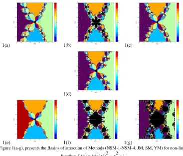
easily judge the stability of iterative methods (MNS-1-MNS-4, JM, SM, YM). Elapsed time, divergent regions and brightness in color presents that MNS-1-MNS-4 is better than JM, SM, and YM.

1(a) 1(b) 1(c)

1(d)

1(e) 1(f) 1(g)

Figure 1(a-g), presents the Basins of attraction of Methods (NSM-1-NSM-4, JM, SM, YM) for non-linear

functionf₁( )x =(sin( ))x 2−x2+1.

Table 2:Elapsed Time for Basin of attraction

f₁xsinx2x21

NSM-1 NSM-2 NSM-3 NSM-4 JM SM YM 19.880778 27.543028 28.366321 35.043862 21.593686 62.496179 61.235432

(7)

2(a) 2(b) 2(c)

2(d)

2(e) 2(f) 2(g)

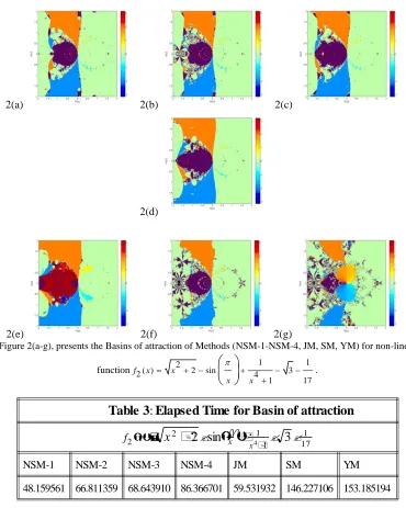
Figure 2(a-g), presents the Basins of attraction of Methods (NSM-1-NSM-4, JM, SM, YM) for non-linear

function ₂( ) 2 2 sin ₄1 3 1

1 17

f x x

x x



= + − + − −

+    

  .

Table 3:Elapsed Time for Basin of attraction

f₂x x2 _₂__sin_

x 

1

x413 1 17

(8)

3(a) 3(b) 3(c)

3(d)

3(e) 3(f) 3(g)

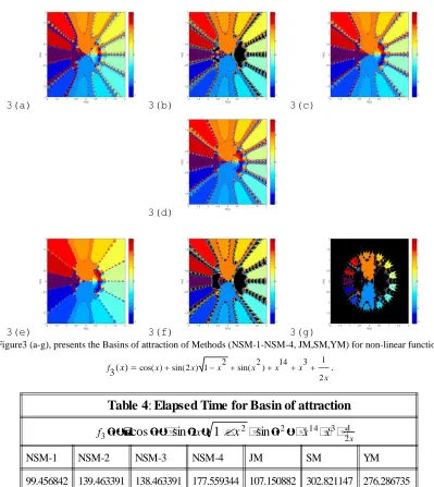
Figure3 (a-g), presents the Basins of attraction of Methods (NSM-1-NSM-4, JM,SM,YM) for non-linear function

1

2 2 14 3

cos( ) sin(2 ) 1 sin( )

2 ( )

3

f x x x x x x x

x = + − + + + + .

Table 4:Elapsed Time for Basin of attraction

f₃xcosxsin2x1x2__sin__x2__x14__x3_1 2x

NSM-1 NSM-2 NSM-3 NSM-4 JM SM YM

99.456842 139.463391 138.463391 177.559344 107.150882 302.821147 276.286735

(9)

4(a) 4(b) 4(c)

4(d)

4(e) 4(f) 4(g)

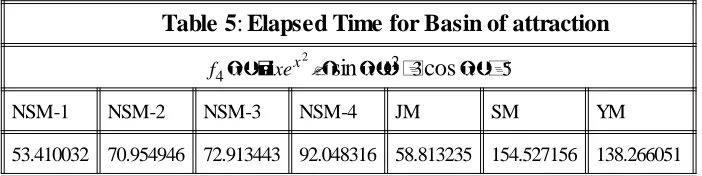
Figure4 (a-g), presents the Basins of attraction of Methods (NSM-1-NSM-4, JM, SM, YM) for non-linear function

2 ₂

4( ) (sin( )) 3cos( ) 5

x

f x =xe − x + x + .

Table 5:Elapsed Time for Basin of attraction

f₄xxex2sinx23cosx5

(10)

Generalization to Simultaneous Iterative

Methods

Suppose, the non-linear equation (1) has n roots. Then f x( ) and f x'( ) can be approximated as:

(

)

(

)

1

1 1

( ) and ( ) .

j

n n n

j j

j k j k

f x x x f x x x

=

= = 



=



− =



− (26)

This implies,

1

1 1 1

( )

( ) 1 1

. ( ) ( ) i j j n n j j

x x x x

j i

f x

f x x x

= = − −   = = − ₋



(27)

This gives, 1 1 1 ( ) ( ) ( ) 1

( ) , where ( ) .

( )

i j

j

i

i i n i

i

N x x x

j i

f x

y x x N x

f x = −  = − =  −



(28)

Now from (27), an approximation of (₍i)₎ i

f x

fx is formed by replacing xj with k xt( j )

 as follows: 1 1 1 ( ) ₍ ₍ ₎₎

( ) 1

, where ( ) , ( 1,..., 4). ( )

i _j i t j

i

t j i

n i

N x _x _{k x}

j i

f x

k x z t

f  x

 =  −  = = = −



(29)

Using (29) in (2), we have: 1 1 1 ( ) ₍ ₍ ₎₎ 1 .( 1,...4)

i _i _t _j

j

i i n

N x _x _{k x}

j i

y x t

 = −  = − = −



(30)

In case of multiple roots 1 1 ( ) ( ( )) .( 1,...4) j

i _i _t _j

j

i

i i n

N x x k x

j i

y x t

   = −  = − = −



(31) where

1 ( ) ( ) 2 1

( ) j ,

j

f y

j j j

f x u

k x z y 

−

= = − (32)

(

( )

)

( )

(

)

(

( )

)

2

2 2 2

1 2

( ) 1 1

( ) ,

( ) 1 1 4 1 1

j

j j j

j

f y u

k x z y

f x u u u

 ₌ ₌ ₋ +

(11)

( )

(

)

3 ₂ 1 2 ( ) ( ) ,

( ) 4 1 1

j

j j j

j

f y

k x z y

f x u u

 ₌ ₌ ₋

+ − (34)

( )

2

4

1 1 1 1

( )

( ) ,

( ) 2

j

j j j

u u

j u

f y

k x z y

f x 

− +

= = −

+ (35)

where ( ) (₍ )₎

( ) and u1=

j i j i f y f x

i i f x

f x

y = −x  .

Using Correction ktx_j_{where t=1,...,4 in (31), we get the following four simultaneous}

iterative methods for extracting all distinct as well as multiple roots of non-linear equation (1).

1 ( ) ₍ ₍ ₎₎ 1 1 ( ) ( ) 1 , , i n j

N xi xikt xj

j j i

i n

j

N yi yi yj

j j i i i i i y x z y      − =  − =  − −  = −    = −   



(36)

where t=1,...4 and j=1,... .n

abbreviated as NMSM-1,NMSM-2,NMSM-3 and NMSM-4.

Convergence Analysis

In this section, the convergence analysis of a family of simultaneous methods (NMSM-1, NMSM-2, NMSM-3 and NMSM-4) given in form of the following theorem. Obviously, convergence for the method (NMSM-1, NMSM-2, NMSM-3 and NMSM-4) will follow from the convergence of the method (NMSM-1, NMSM-2, NMSM-3 and NMSM-4) from theorem (2) when the multiplicities of the roots are simple.

Theorem: Let 1,2, . . . ,n be the n number of simple roots of non-linear equation (1). If

x₁0,_x₂0,_x₃0, . . . ,_xn0 be the initial approximations of the roots respectively and

sufficiently close to actual roots, the order of convergence of methods (NMSM-1, NMSM-2, NMSM-3 and NMSM-4) equals twelve.

Proof Let

_i = −x_i  _i, _i' = y_i−_i and _i'' = −z_i _i (37) be the errors in xi and yi approximations respectively. Considering (NMSM-1, NMSM-2,

NMSM-3 and NMSM-4), which is

1

( ) ₍ ₍ ₎₎

, ( 1,..., 4).

j i

i i t j

j

i

i i n

N x _x _{k x}

j i

y x t

    = −  = − = −



(38) where ( ) ( ) . ( ) i i i f x N x f x = 

(12)

1

1 ( )

1 1 1 1

.

( ) ( ) ( ) ( ) ( )

j

n n

i

j j i

i i i j i i i j

f x

N x f x x  x  x 

=

= 



= = = +

− − −



(39)

Thus, for multiple roots we have from (NMSM-1, NMSM-2, NMSM-3 and NMSM-4):

1 1 ( ) ( ) ( ( )) , j j i

i i i j _i _t _j

j j

i

i i n n

x x x k x

j i j i

y x        = = − − ₋   = − +



−



(40) 1 ( ( ) ) ( ) ( )( ( )) ,

j i t j i j

i

i i i j i t j

j

i

i i i i n

x k x x

x x x k x

j i y x     _      = − − + − − −  − = − − +



(41) 1 ( ) ( )( ( )) ,

j j j

i

i i j i t j

j

i

i i n

x

x x k x

j i     _      =  − − − −  = − +



(42)

(

)

(

)

(

)

1 , ( ) ( ) j i i i n

j t j j

i i

j i i j i t j

k x

x x k x

        =    = − − − + − −



(43) 1 2 . , j i i i n

i i i j

j i E       =  = − +



(44)

where k xt( j ) j 4j

 ₋ ₌

from (9) and

( )( ( )).

j

i j i t j

i _x _x _{k x}

E _  

− − − = Thus, 1 1 2 4 2 . j j n

i i j

j i

i n

i i i j

j i E E        ₌ =   = +



(45)

If it is assumed that absolute values of all errors _j (j=1, 2, 3,...) are of the same order as, say_j =O , then from (45), we have:

_i =O( ) . 6 (46)

Now consider second step of method (NMSM-1, NMSM-2, NMSM-3 and NMSM-4) and using zi i i

❖❖

, yi i i ❖

(13)

( ) ₍ ₎ 1 . j i

i i j

j

i

i i n

N y _{j i} y y

     =  −        = −  _{− }      (47)

Now, from 2nd_{-step of (NMSM-1, NMSM-2, NMSM-3 and NMSM-4) , we have:}

1 1

( ) ( )

j j

i

i j i j

i

j j

i

i i n n

y y y

j i j i

         = =  − −   = − +



−



(48) 1 ( ) ( )( ) ,

j j j

i j i j

j

i i i

n y

i i y y y

j i         =   − − − −  = −     + _ _ 



 (49) 1 1 2 ( )

, where .

( )( )

j

n

i j i

j i

j i

n

i j i j

i i j i

j i

S

y y y

S          =   =           ₋   = = − − +



Since, _i =O( ) 6 from (46), thus,

( )

2

6 12

''

.

i O O

 =  =  (50)

Thus from (50),i O( ) 12 

= , shows convergence order of method (NMSM-1, NMSM-2, NMSM-3 and NMSM-4) are twelve. Hence prove the theorem.

Computational Aspect

Here, we compare the computational efficiency of the Midrog Petkovic method [8] and the new method(NMSM-1, NMSM-2, NMSM-3, NMSM-4). As presented in [8], the efficiency of an iterative method can be estimated using the efficiency index given by

EL m( )=logr,

D (51)

where D is the computational cost and r is the order of convergence of the iterative method. Using arithmetic operation per iteration with certain weight depending on the execution time of operation to evaluate the computational cost D . The weights used for division,

multiplication and addition plus subtraction are w d, w m, w AS respectively. For a given

(14)

subtraction per iteration for all roots are denoted by D m , M m and AS m . The cost of

computation can be calculated as:

D=D( )m =w AS_as _m+w M_m _m+w D_d _m, (52) thus (51) becomes:

( ) log

as m m m d m

EL m

w AS w M w D

=

+ +

r

(53) Considering the number of operations of a complex polynomial with real and complex roots reduce to operation of real arithmetic, given in Table 3.1 as polynomial degree m taking the dominants term of order m2_{. Apply (4.3) and data given in Table 6, we calculate the} percentage ratio ((NMSM− −1 NMSM−4), ( ))X [8 given by:

( )

(( 1 ), ( )) 1 4 1 100

)

4 ,

(

NMSM NMSM

NMSM N X EL

E SM

L M

X

 =_ − − − − _

 

− − − (54)

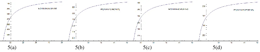
where X is one of the methods, namely Elirch-Aberth and Petkovic methods. Figure 4.1 graphically illustrates these percentage ratioes. It is evident from figure 4.1 that the newly constructed simultaneous methods (3.11,3.12,3.13,3.14) is more efficient as compared to the Elirch [14] and Petkovic methods [8,13].

Table 6:The number of basic operations

Methods CO ASm Mm Dm NMSM-1 12 5m2O(m) 2m2O(m) 2m2O(m) NMSM-2 12 8m2O(m) 3m2O(m) 2m2O(m) NMSM-3 12 7m2O(m) 2m2O(m) 2m2O(m) NMSM-4 12 5m2O(m) 2m2O(m) 2m2O(m) PJ10D 10 22m2O(m) 18m2O(m) 2m2O(m)

We also calculate the CPU execuation time, as all the calculations are done using maple 18 on (Processor Intel(R) Core(TM) i3-3110m [email protected] with 64-bit Operating System. We observe that CPU time of the method MMN8M is less than M. S. Petkovic methods [8], showing the domminace efficiency of our method 3.11,3.12,3.13,3.14 as compared to them.

5(a) 5(b) 5(c) 5(d)

(15)

Numerical Results

Here, some numerical examples are considered in order to demonstrate the performance of our family of two-step fourth order single root finding methods (NMS-1,NMS-2,NMS-3,NMS-4) and two-step twelfth order simultaneous methods (NMSM-2,NMSM-2,NMSM-3,NMSM-4) respectively. We compare our family of single root finding methods with optimal fourth order method JM,YM and SM. Family of simultaneous methods of order twelve are compare with J. Džunic, M. S. Petkovic and L. D. Petkovic [8] method of order ten (abbreviated as PJ10D method). All the computations are performed using Maple 18 with 2500 (64 digits floating point arithmetic in case of simultaneous methods) significant digit with stopping criteria is as follow.

i ei  f x_i

k1

, ii ei  x_i

k1

_i

2

,

where ei represents the absolute error of function values in i and norm-2 in ii [8].

We take 10200 for single root finding method and 1030 for simultaneous determination of all roots of non-linear equation ().

Numerical tests examples from [10, 14, 15, 17, 23] are provided in Tables 7(a, b) and 8-13 .In Table 8-13 the stopping criteria ( )i is used while in Table 7(a, b) the stopping criteria (i) and (ii) both are used. In all Tables CO represents the convergence order, n represents the number of iterations,  =1 represents all distinct root,  1 represents multiple rootsand CPU represents computational time in seconds. We observe that numerical results of the methods (in case of single (NMS-1, NMS-2, NMS-3, NMS-4) as well as simultaneous determination (NMSM-2, NMSM-2, NMSM-3, NMSM-4) of all roots) are better than JM, YM SM and PJ10D respectively on same number of iterations. The Figure 7(a-d) and 8(a, b)-13(a, b), shows the residual fall of different methods for the non-linear function f x f x f₁( ), ₂( ), ₃(x) , ( )f x₄ and examples 4.1,4.2,4.3,4.4,4.5,4.6 (in case of simultaneous methods), shows that methods (NMS-1,NMS-2,NMS-3,NMS-4) and (NMSM-2,NMSM-2,NMSM-3,NMSM-4) are more efficient as compared than JM, YM SM and PJ10D respectively.

2 2 1

( )... ( )[23]i f x =(sin( ))x −x +1, =1.4044916482.

2

2 4

1 1

( )... ( )[17] 2 sin 3 , 2 1 17

ii f x x

x x

 _

 

= + − _{ }+ − − = − +

 

2 2 14 3

3

1

( )... ( )[23] cos( ) sin(2 ) 1 sin( ) , 0.9257722498 2

iii f x x x x x x x

x 

= + − + + + + = −

2 ₂

4

( )... ( )[23] x (sin( )) 3cos( ) 5, 1.207647827130919

(16)

6(a) 6(b) 6(c) 6(d) 6(e)

6(f) 6(g)

Table.7(a):Comparsion of optimal Fourth order methods

Initial guesses |fixi| CPU CO n JM SM AM NMS-1 NMS-2 NMS-3 NMS-4

f1, x0 1. 5 |f1x6| 4 6 4.3e-90 div 1.4e-58 1.3e-697 1.6e-700 2.0e-700 2.9e-700

CPU forf1 0.125 0.109 .110 0.125 0.125 0.109

f2, x0 2. 25 |f2x6| 4 6 8.0e-90 div 2.5e-48 1.0e-931 2.1e-886 2.6e-884 1.5e-880

CPU forf2 0.111 0.125 0.125 0.125 0.125 0.141

f3, x0 0. 93 |f3x6| 4 6 8.5e-117 div 3.1e-83 8.8e-1011 1.7e-1011 1.7e-1011 1.8e-1011

CPU forf3 0.250 0.234 0.234 0.250 0.250 0.266

f4, x0 1. 3 |f4x6| 4 6 4.7e-71 div 2.8e-43 2.5e-541 1.4e-540 1.3e-540 1.1e-540

(17)

Table.7(b):Comparsion of optimal Fourth order methods

Initial guesses x_ik1☺ CO n JM SM AM NMS-1 NMS-2 NMS-3 NMS-4

f1, x0 1. 5 xi 6

☺ 4 6 4.4e-90 div 6.0 e-30 3.1e-233 3.4e-234 3.6e-234 4.1e-234

CPU forf1 0.125 0.109 .110 0.125 0.125 0.109

f2, x0 2. 25 xi 6

☺ 4 6 8.3e-45 div 2.3e-24 2.0e-310 2.6e-295 1.3e-294 2.3e-293

CPU forf2 0.111 0.125 0.125 0.125 0.125 0.141

f3, x0 0. 93 xi 6

☺ 4 6 1.9e-591 div 6.2e-43 2.4e-338 1.4e-338 1.4e-338 1.4e-338

CPU forf3 0.250 0.234 0.234 0.250 0.250 0.266

f4, x0 1. 3 xi 6

☺ 4 6 1.6e-36 div 6.8e-23 1.4e-181 2.5e-181 2.5e-181 2.3e-181

CPU forf4 0.140 0.141 0.141 0.141 0.156 0.140

7(a) 7(b) 7(c)

(18)

Example 4.1[15]: Consider

2 3 2 2 2 2 3 2

5( ) ( +1) ( +2) ( -2 +2) ( +1) ( -2) ( +2i) ,

f x = x x x x x x x

with multiple exact roots ( 1):

1 1, 2 2, 3,4 2i, 5,6 i, 7 2, 8 2i.

The initial approximations have been taken as:

0

x1  1. 3. 2i,

0

x22. 2. 3i,

0

x 3 1. 31. 2i,

0

x 4 0. 71. 2i,

0

x 5 0. 2. 8i,

0

x 6 0. 21. 3i,

0

x 7 2. 2. 3i,

0

x 8 2. 20. 7i.

For distinct roots ( 1_):

2 2

( ) ( +1) ( +2) ( -2 +2) ( +1) ( -2) ( +2i).

f x = x x x x x x x

Table.8

Method CO CPU  n e1 e2 e3 e4 e5 e6 e7 e8

PJ10D 10 0.766 1 2 1.2e-1 3.0e-2 2.7e-1 7.9e-2 1.8e-1 3.1e-2 1.2e-1 8.2e-3

NMSM(1-4) 12 0.250 1 2 1.9e-36 1.8e-36 0.0 0.0 1 2e-39 3.8e-37 3.5e-37 0.0

NMSM(1-4) 12 0.328 1 2 2.0e-58 1.0e-51 0.0 6.4e-81 2.6e-120 1.5e-82 1.6e-51 3.8e-69

8(a) 8(b)

Example4.2[15]: Consider

3 2 3 3

6( ) ( +1) ( +2) ( -1-i) ( -1+i) ,

f x = x x x x

1 1, 2 2, 3 1i, 4 1i.

(19)

0

x11. 10. 2i,

0

x22. 1. 2i,

0

x 3 0. 81. 2i,

0

x 4 0. 91. 2i.

For distinct roots ( 1 ):

( ) ( +1) ( +2) ( -1-i)( -1+i)

f x = x x x x

Table.9

Method CO CPU  n e1 e2 e3 e4

PJ10D 10 0.047 1 2 5.9e-22 3.4e-22 5.9e-22 4.2e-22

NMSM(1-4) 12 0.032 1 2 3.8e-95 1.9e-93 0.0 0.0

NMSM(1-4) 12 0.032 1 2 3.0e-129 2.5e-197 0.0 0.0

9(a) 9(b)

Example4.3[14]: Consider

(

₍ _{1) (} _{2) (} ₃₎

)

5

7( ) 1 ,

x x x x

f x = e − − − −

1 0, 2 1, 3 2, 4 3.

0

x10. 1,

0

x20. 9,

0

x 3 1. 8,

0

x 4 2. 9,

(20)

Table.10

Method CO CPU  n e1 e2 e3 e4

PJ10D 10 0.156 1 2 9.3e-3 2.7e-4 1.2e-3 9.3e-3

NMSM(1-4) 12 0.078 1 2 1.0e-9 0.0 0.0 2.1e-9

NMSM(1-4) 12 0.078 1 2 0.0 0.0 0.0 8.1e-27

10(a) 10(b

(

)

(

)

5

3 2 3 2

8( ) +5 -4 -20+ cos +5 -4 -20 -1 ,

f x = x x x x x x

1 - 5, 2 - 2, 3 2,

0

x15. 1,

0

x21. 8,

0

x 3 1. 9.

fxx3_₅_x2_-4_x_-20__cos _x 3_₅_x2_-4_x_{-20 -1.}

Table.11

Method CO CPU  n e1 e2 e3

PJ10D 10 0.187 1 2 4.9e-3 6.0e-3 2.5e-1

NMSM(1-4) 12 0.094 1 2 7.2e-11 1.7e-10 2.3e-4

(21)

11(a) 11(b

3 3 3

9

1 2 2.5

( ) sin sin sin ,

2 2 2

x x x

f x = _ − _ _ − _ _ − _

     

1 0, 2 1, 3 2, 4 3.

0

x10. 1,

0

x20. 9,

0

x 3 1. 8,

0

x 4 2. 9.

fxfxsin x 1

2 sin

x 2

2 sin

x2. 5

2 .

Table.12

Method CO CPU  n e1 e2 e3

PJ10D 10 0.312 1 2 6.4e-3 1.0e-3 1.6e-4

NMSM(1-4) 12 0.140 1 2 3.0e-3 1.0e-17 1.3 e-13

NMSM(1-4) 12 0.109 1 2 1.6e-3 1.6e-34 6.9e-53

12(a) 12(b

(22)

5 5 10

2 3

( ) sinh sinh

2 2

x x

f x = _ + _ _ − _

   

1 0, 2 1, 3 2, 4 3.

0

x10. 1,

0

x20. 9,

0

x 3 1. 8,

0

x 4 2. 9.

fxsinh x 2

2 sinh

x 3 2

Table.13

Method CO CPU  n e1 e2

PJ10D 10 0.047 1 2 6.4e-3 1.0e-3

NMSM(1-4) 12 0.016 1 2 1.2e-8 1.0e-7

NMSM(1-4) 12 0.030 1 2 1.2e-36 1.4e-38

13(a) 13(b

Conclusion

(23)

References

[1] M. Cosnard and P. Fraigniaud, Finding the roots of a polynomial on an MIMD multicomputer, Parallel Computing, vol. 15, no. 1--3, (1990), 75--85.

[2] S. Kanno, N, Kjurkchiev, T. Yamamoto, On some methods for the simultaneous determination of polynomial zeros, Japan J. Apple. Math. 13(1995), 267-288.

[3] O. Abert, Iteration methods for finding all zeros of a polynomial simultaneously, Math. Comput. 27(1973) 339-344.

[4] P.D. Proinov, S.I. Cholakov, Semilocal convergence of Chebyshev-like root-finding method for simultaneous approximation of polynomial zeros, Appl. Math. Comput. 236(2014), 669-682.

[5] Bl. Sendov, A. Andereev and N. Kjurkchiev, Numerical Solutions of polynomial Equations, Elsevier science, New York, 1994.

[6] X. Wang, L. Liu, Modified Ostrowski's method with eight --order convergence and high efficiency index, Applied Mathematics Letters, 23(2010), 549-554.

[7] T.-F. Li, D.-S. Li, Z.-D.Xu, and Y.-I. Fang, New iterative methods for non-linear equations, Applied Mathematics and Computations,.(2008), 755-759.

[8] M.S.Petkovi´c, L.D.Petkovic, J.Džunic, On an efficient simultaneous method for finding polynomial zeros, Appl. Math. Lett. 28(2014), 60-65.

[9] P.D. Proinov, M.T. Vasileva, On the convergance of family of Weierstrass-type root-finding methods, C. R. Acad. Bulg. Sci, 68(2015), 697-704.

[10] N. A. Mir, R. Muneer, I. Jabeen, Some families of two-step simultaneous methods for determining zeros of non-linear equations,ISRN Applied Mathematics, (2011), 1-11. [11] P.D. Proinov, S.I. Cholakov, Semilocal convergence of Chebyshev-like root-finding

method for simultaneous approximation of polynomial zeros, Appl. Math. Comput. 236(2014), 669--682.

[12] M.S.Petkovic, L.D.Petkovic, J.Džunic, On an efficient simultaneous method for finding polynomial zeros, Applied Mathematics Letters, 28(2014), 60-65.

[13] O. Aberth, Iteration methods for finding all zeros of a polynomial simultaneously, Math. Comp. 27(1973) 339-344.

[14] G. H. Nedzhibov, Iterative methods for simultaneous computing arbitrary number of multiple zeros of nonlinear equations, International Journal of Computer Mathematics, (2013), 994-1007.

[15] M.R. Farmer, Computing the zeros of polynomials using the divide and Conquer approach, Ph.D Thesis, Department of Computer Science and Information Systems, Birkbeck, University of London, July 2014.

[16] I.K. Argyros, D. Chen, Q. Qian. The Jarratt method in Banach space setting. J. Comput. Appl. Math. 51, pp. 103-106, 1994.

[17] H. I. Siyyam, I.A. Al-Subaihi. A new class of optimal fourth-order iterative methods for solving nonlinear equations, European Journal of Scientific Research. 109, 2, pp.

224-231, 2013.

[18] Osama Y. Ababneh, New fourth order iterative methods second derivative free, J. Appl. Math. Phy. 2016, 4, 519-523

(24)

[20] A.Cordero, J. García-Maimó, J.R. Torregrosa, M.P. Vassileva, P. Vindel, Chaos in King's iterative family, Appl. Math. Lett. 26 (2013), 842--848.

[21] F. Chicharro, A. Cordero, J.R. Torregrosa, Drawing dynamical and parameters planes of iterative families and methods, Sci. World J. 2013 (2013).

[22] A. W. M. Nourein, An improvement on two iteration methods for simultaneous

determination of the zeros of a polynomial, Inrern. J. Cornput. Math. (1977), 241--252. [23] F. Soleymani, Optimal fourth-order iterative methods free from derivatives, Miskolc

Mathematical Notes, vol. 12 (2011), no. 2, 255–264.

[24] P.D. Proinov, A general semilocal convergence theorem for simultaneous methods for polynomial zeros and its applications to Ehrlich's and Dochev-Byrnev's methods, Appl. Math. Comput. 284 (2016), 102--114.

[25] Jay, L.O. A note on Q-order of convergence. BIT Numer. Math. 2001, 41, 422--429. [26] P.D. Proinov, S.I. Ivanov, On the convergence of Halley's method for simultaneous

computation of polynomial zeros, J. Numer. Math. 23 (2015), 379--394.

[27] P.D. Proinov, S.I. Ivanov, Convergence analysis of Sakurai-Torii-Sugiura iterative

method for simultaneous approximation of polynomial zeros, J. Comput. Appl. Math. 357 (2019), 56--70.

[28] S.I. Cholakov, Local and semilocal convergence of Wang-Zheng's method for simultaneous finding polynomial zeros, Symmetry 2019 (2019), Art. 736, 15pp. [29] M. Dehghan, M. Hajarian, On derivative free cubic convergence iterative methods for

solving nonlinear equations, Comput. Math. Math. Phy. 51(2011), 513-519. [30] M. Dehghan, M. Hajarian, On some cubic convergence iterative formulae without

derivatives for solving nonlinear equations. Int. J. Numer. Meth. Biomed. Eng. Vol. 27, 27(2011), 722-731.

Creative Commons CC BY